Statistical Reasoning for Everyday Life (5th Edition)
5th Edition
ISBN: 9780134494043
Author: Jeff Bennett, William L. Briggs, Mario F. Triola
Publisher: PEARSON
expand_more
expand_more
format_list_bulleted
Concept explainers
Videos
Textbook Question
Chapter 7, Problem 6CRE
Pizza and the Subway. For Exercises 1–6, refer to the following table that lists the cost (in dollars) of a slice of pizza in New York City and the subway fare in the same year.
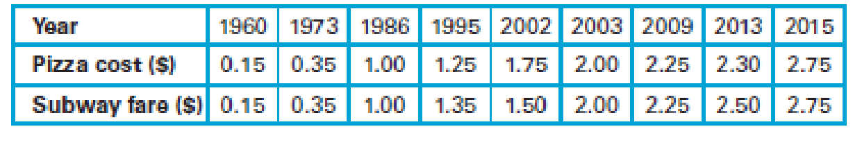
6. Using the equation for the best-fit line, we find that when a slice of pizza costs $1000, the predicted subway fare is $1011. Is that predicted subway fare likely to be an accurate prediction? Why or why not?
Expert Solution & Answer
Want to see the full answer?
Check out a sample textbook solution
Students have asked these similar questions
In Exercises 37–40, determine the value of k.
Complete Part D
A recent issue of the AARP Bulletin reported that the average weekly pay for a woman with a high school degree is $520 (AARP Bulletin, January–February, 2010). Suppose you would like to determine if the average weekly pay for all working women is significantly greater than that for women with a high school degree. Data providing the weekly pay for a sample of 50 working women are available in the file named WeeklyPay. These data are consistent with the findings reported in the AARP article. Complete D
null hyposthesis: H(o)=520Alternative hypothesis: H(a): greater then 520
sample mean=637.94
the test statistic = 5.62
p-value=0.00
Using a=.05, we would reject the null hypothesis.
D. Repeat the hypothesis test using the critical value approach.
582
333
759
633
629
523
320
685
599
753
553
641
290
800
696
627
679
667
542
619
950
614
548
570
678
697
750
569…
For Exercises 34 – 36, use the following information. Soto wants to enlarge a digital photograph that is 1800 pixels wide and 1600 pixels high (1800 x 1600) by a scale factor of
34. What will be the dimensions of the new digital photograph?
Chapter 7 Solutions
Statistical Reasoning for Everyday Life (5th Edition)
Ch. 7.1 - Correlation. What is a correlation? Give three...Ch. 7.1 - Scatterplot. What is a scatterplot, and how is one...Ch. 7.1 - Types of Correlation. Define and distinguish...Ch. 7.1 - Correlation Coefficient. What does the correlation...Ch. 7.1 - Does It Make Sense? For Exercises 58, determine...Ch. 7.1 - Does It Make Sense? For Exercises 58, determine...Ch. 7.1 - Does It Make Sense? For Exercises 58, determine...Ch. 7.1 - Does It Make Sense? For Exercises 58, determine...Ch. 7.1 - Correlation. Exercises 916 list pairs of...Ch. 7.1 - Correlation. Exercises 916 list pairs of...
Ch. 7.1 - Correlation. Exercises 916 list pairs of...Ch. 7.1 - Correlation. Exercises 916 list pairs of...Ch. 7.1 - Correlation. Exercises 916 list pairs of...Ch. 7.1 - Correlation. Exercises 916 list pairs of...Ch. 7.1 - Correlation. Exercises 916 list pairs of...Ch. 7.1 - Correlation. Exercises 916 list pairs of...Ch. 7.1 - Crickets and Temperature. One classic example of a...Ch. 7.1 - Two-Day Forecast. Figure 7.8 shows a scatterplot...Ch. 7.1 - Properties of the Correlation Coefficient. For...Ch. 7.1 - Properties of the Correlation Coefficient. For...Ch. 7.1 - Properties of the Correlation Coefficient. For...Ch. 7.1 - Properties of the Correlation Coefficient. For...Ch. 7.1 - Scatterplot and Correlation. In Exercises 2330,...Ch. 7.1 - Scatterplot and Correlation. In Exercises 2330,...Ch. 7.1 - Scatterplot and Correlation. In Exercises 2330,...Ch. 7.1 - Prob. 26ECh. 7.1 - Scatterplot and Correlation. In Exercises 2330,...Ch. 7.1 - Scatterplot and Correlation. In Exercises 2330,...Ch. 7.1 - Scatterplot and Correlation. In Exercises 2330,...Ch. 7.1 - Scatterplot and Correlation. In Exercises 2330,...Ch. 7.1 - Your Own Positive Correlations. Give examples of...Ch. 7.1 - Your Own Negative Correlations. Give examples of...Ch. 7.2 - Outliers. Briefly explain how an outlier can make...Ch. 7.2 - Grouped Data. Briefly explain how data that...Ch. 7.2 - Explanations for Correlation. What are the three...Ch. 7.2 - Prob. 4ECh. 7.2 - Does It Make Sense? For Exercises 58, determine...Ch. 7.2 - Does It Make Sense? For Exercises 58, determine...Ch. 7.2 - Does It Make Sense? For Exercises 58, determine...Ch. 7.2 - Does It Make Sense? For Exercises 58, determine...Ch. 7.2 - Correlation and Causality. Exercises 916 present...Ch. 7.2 - Correlation and Causality. Exercises 916 present...Ch. 7.2 - Correlation and Causality. Exercises 916 present...Ch. 7.2 - Correlation and Causality. Exercises 916 present...Ch. 7.2 - Correlation and Causality. Exercises 916 present...Ch. 7.2 - Correlation and Causality. Exercises 916 present...Ch. 7.2 - Correlation and Causality. Exercises 916 present...Ch. 7.2 - Correlation and Causality. Exercises 916 present...Ch. 7.2 - Outlier Effects. Consider the scatterplot in...Ch. 7.2 - Outlier Effects. Consider the scatterplot in...Ch. 7.2 - Footprint and Height. The following table lists...Ch. 7.2 - January and July High Temperatures. The following...Ch. 7.2 - Birth and Death Rates. Figure 7.17 shows the birth...Ch. 7.2 - Penny Weight and Date. The scatterplot in Figure...Ch. 7.3 - Best-Fit Line. What is a best-fit line? How is a...Ch. 7.3 - Prob. 2ECh. 7.3 - Interpreting r2. What does the square of the...Ch. 7.3 - Prob. 4ECh. 7.3 - Prob. 5ECh. 7.3 - Does It Make Sense? For Exercises 58, determine...Ch. 7.3 - Does It Make Sense? For Exercises 58, determine...Ch. 7.3 - Does It Make Sense? For Exercises 58, determine...Ch. 7.3 - Best-Fit Lines. Exercises 916 refer to tables in...Ch. 7.3 - Best-Fit Lines. Exercises 916 refer to tables in...Ch. 7.3 - Prob. 11ECh. 7.3 - Best-Fit Lines. Exercises 916 refer to tables in...Ch. 7.3 - Best-Fit Lines. Exercises 916 refer to tables in...Ch. 7.3 - Best-Fit Lines. Exercises 916 refer to tables in...Ch. 7.3 - Prob. 15ECh. 7.3 - Prob. 16ECh. 7.4 - Correlation and Causality. What is the difference...Ch. 7.4 - Prob. 2ECh. 7.4 - Establishing Causality. Briefly state in your own...Ch. 7.4 - Confidence in Causality. Describe three levels of...Ch. 7.4 - Prob. 5ECh. 7.4 - Does It Make Sense? For Exercises 58, determine...Ch. 7.4 - Does It Make Sense? For Exercises 58, determine...Ch. 7.4 - Does It Make Sense? For Exercises 58, determine...Ch. 7.4 - Physical Models. For Exercises 912, determine...Ch. 7.4 - Physical Models. For Exercises 912, determine...Ch. 7.4 - Physical Models. For Exercises 912, determine...Ch. 7.4 - Physical Models. For Exercises 912, determine...Ch. 7.4 - Altitude and Health. When some people climb to...Ch. 7.4 - Smoking and Lung Cancer. There is a strong...Ch. 7.4 - Other Lung Cancer Causes. Several things besides...Ch. 7.4 - Longevity of Orchestra Conductors. A famous study...Ch. 7.4 - Older Moms. A study reported in Nature claims that...Ch. 7.4 - High-Voltage Power Lines. Suppose that people...Ch. 7.4 - Gun Control. Those who favor gun control often...Ch. 7.4 - Vasectomies and Prostate Cancer. The article Does...Ch. 7 - Pizza and the Subway. For Exercises 16, refer to...Ch. 7 - Pizza and the Subway. For Exercises 16, refer to...Ch. 7 - Pizza and the Subway. For Exercises 16, refer to...Ch. 7 - Pizza and the Subway. For Exercises 16, refer to...Ch. 7 - Pizza and the Subway. For Exercises 16, refer to...Ch. 7 - Pizza and the Subway. For Exercises 16, refer to...Ch. 7 - For 10 pairs of sample data values, the...Ch. 7 - In a study involving randomly selected subjects,...Ch. 7 - A researcher collects paired sample data values...Ch. 7 - Estimate the value of the linear correlation...Ch. 7 - Fill in the blanks: Every possible correlation...Ch. 7 - Which of the following are likely to have a...Ch. 7 - For a collection of 50 pairs of sample data...Ch. 7 - Estimate the correlation coefficient for the data...Ch. 7 - Refer again to the scatterplot in Figure 7.24....Ch. 7 - Fill in the blank: If r = 0.900, then _____ % of...Ch. 7 - In Exercises 710, determine whether the given...Ch. 7 - Prob. 8CQCh. 7 - Prob. 9CQCh. 7 - Prob. 10CQ
Knowledge Booster


Learn more about
Need a deep-dive on the concept behind this application? Look no further. Learn more about this topic, statistics and related others by exploring similar questions and additional content below.Similar questions
- Page of 11 ZOOM + 5. The table shows how the cost of a carne asada taco at my favorite taco stand has increased as they have become more popular since their opening in 2013. Use the data to answer the questions below. Year, x 2013, 0 2014, 1 2015, 2 2016, 3 2017, 4 2018, 5 2019,6 Cost ($) 0.50 0.55 0.65 0.75 0.90 1.00 1.10 (a) What is the regression line given by your TI-84 for this data? Round values to 3 decimal places. (b) Using the regression equation above, predict the cost of a carne asada taco at my favorite taco stand in 2020. Show the work.arrow_forwardLarge companies typically collect volumes of data before designing a product, not only to gain information as to whether the product should be released, but also to pinpoint which markets would be the best targets for the product. Several months ago, I was interviewed by such a company while shopping at a mall. I was asked about my exercise habits and whether or not I'd be interested in buying a video/DVD designed to teach stretching exercises. I fall into the male, 18 – 35-years-old category, and I guessed that, like me, many males in that category would not be interested in a stretching video. My friend Diane falls in the female, older-than-35 category, and I was thinking that she might like the stretching video. After being interviewed, I looked at the interviewer's results. Of the 93 people in my market category who had been interviewed, 17 said they would buy the product, and of the 113 people in Diane's market category, 34 said they would buy it. Assuming that these data came…arrow_forwardLarge companies typically collect volumes of data before designing a product, not only to gain information as to whether the product should be released, but also to pinpoint which markets would be the best targets for the product. Several months ago, I was interviewed by such a company while shopping at a mall. I was asked about my exercise habits and whether or not I'd be interested in buying a video/DVD designed to teach stretching exercises. I fall into the male, 18 – 35-years-old category, and I guessed that, like me, many males in that category would not be interested in a stretching video. My friend Amanda falls in the female, older-than-35 category, and I was thinking that she might like the stretching video. After being interviewed, I looked at the interviewer's results. Of the 97 people in my market category who had been interviewed, 16 said they would buy the product, and of the 101 people in Amanda's market category, 31 said they would buy it. Assuming that these data came…arrow_forward
- I’m taking a probability and statistics math class. Please get this correct so I can study.arrow_forwardThe university wants to know if Annual Income and Lifetime Savings are linearly related. Investigate and state your answer with evidence. Does your answer seem logical or not? Write your thoughts on this.arrow_forwardi only want part D to be solvedarrow_forward
- Answer completely and neatly. Show detailed solutions.arrow_forwardThe bar graph shows the average cost of tuition and fees at private four-year colleges in a particular country. Below are two mathematical models for the data shown in the graph. In each formula, T represents the average cost of tuition and fees at private colleges for the school year ending x years after 2000. Answer parts a and b. Average Cost of Tuition and Fees at Private Four-Year Colleges 22 20- 22,051 21,057 20,095 19,128 18,135 18- 16.203 16 15 218 17,168 Model 1 T= 974x+ 15,223 Model 2 T= - 2.1x + 988x + 15,208 14 2000 2001 20022003 2004 2005 2006 2007 a. Use each model to find the average cost of tuition and fees at private colleges for the school vear ending in 2003. By how much does each model underestimate or overestimate the actual cost shown for the school year ending in 2003? HIHE The average cost given by model 1 is $ Round to the nearest dollar.) Help Me Solve This Textbook Get More Help - Clear All Skill Builder Check Answer 10.19 PM 65°F 9/6/2021 Type here to search…arrow_forward21–23. Language enrollments. The line graph in Figure 2.28 shows total course enrollments in languages other than English in U.S. institutions of higher education from 1960 to 2009. (Enrollments in ancient Greek and Latin are not included.) Exercises 21 through 23 refer to this figure. 1,800,000 1,629,326 1.522.770 1,600,000 - 1,400,000 - 1347.036 1,200,000- 1,073,097 1,067,217 1,000.000 - 975.7m 963,930 883.222 1.06.603 922,439 960.588 B00,000 - 97.077 877.91 600,000 - 608,749 400.000 - 200,000 - 1960 1965 1968 | 1972 1977 1980 1983 1986 1990 1995 199 2002 2006 2009 1970 1974 Figure 2.28 Crauder, et al., Quantitative Literacy, 3e, © 2019 W. H. Freeman and Company FIGURE 2.28 Enrollments in languages other than English in U.S. institutions of higher education (2009). 21. During which time periods did the enrollments decrease? 22. Calculate the average growth rate per year in enrollments over the two periods 1960–1965 and 2006– 2009. Note that the time periods are not of the same…arrow_forward
- Research suggests that spending time with animals can reduce blood pressure. I want to know whether particular animals are better at reducing blood pressure than others. I randomly select 10 participants. Each participants' blood pressure is measured when they enter the lab (Time 1; baseline). Participants' blood pressure is then measured again after they spend a half-hour with a dog. Lastly, participants' blood pressure is measured a third time after they spend a half-hour with a cat. 1. How many levels of the IV are there? A. 3 B. 2 C. 4 D. 1 2. Is the scenario above between- or within-subjects? A. Within-Subjects B. Between-Subjects 3. What test would be used to analyze the scenario above? A. One-Way Repeated Measures ANOVA B. One-Way Between-Subjects ANOVA C. Independent Groups t-test D. Correlated Groups t-testarrow_forwardlecture(11.14): A professor offered a course that was offered half online and half in person. The professor hypothesized that students were spending less time on the material than on the off line material. At the end of the semester, students were asked to provide the amount of time they tended to course tasks during a week. The weeks were classified as online or in person, and the average amount of time is provided for 15 students. Online: 4 3 5 6 2 2 4 7 5 4 3 2 6 6 3 In person: 5 5 4 7 3 4 4 6 4 5 3 4 5 8 4 Test the hypothesis at( alpha=0.05) level of significance using the 5 step procedure. Make sure to clearly state the null and alternative hypothessis. Round your answer to 2 decimal places.arrow_forward9.The equation shown is a model developed by a researcher, where x represents the height, in inches, of a 36-month-old boy and y represents his maximum height, in inches, as an adult. y = 3.5x - 60 Part A A 36-month-old boy has a height of 36 inches. Based on the model, what is his expected height, in inches as an adult? Part B Jack and Kris are 36-month old boys. Jack is exactly 1.5 inches taller than Kris. Based on the model, how many inches taller is Jack expected to be than Kris is expected to be when they are adults? Part C An adult male has a height of 80 inches, Based on the model, what was his height, in inches, when he was 36 monthsarrow_forward
arrow_back_ios
SEE MORE QUESTIONS
arrow_forward_ios
Recommended textbooks for you
 MATLAB: An Introduction with ApplicationsStatisticsISBN:9781119256830Author:Amos GilatPublisher:John Wiley & Sons Inc
 Probability and Statistics for Engineering and th...StatisticsISBN:9781305251809Author:Jay L. DevorePublisher:Cengage Learning
 Statistics for The Behavioral Sciences (MindTap C...StatisticsISBN:9781305504912Author:Frederick J Gravetter, Larry B. WallnauPublisher:Cengage Learning
 Elementary Statistics: Picturing the World (7th E...StatisticsISBN:9780134683416Author:Ron Larson, Betsy FarberPublisher:PEARSON
 The Basic Practice of StatisticsStatisticsISBN:9781319042578Author:David S. Moore, William I. Notz, Michael A. FlignerPublisher:W. H. Freeman
 Introduction to the Practice of StatisticsStatisticsISBN:9781319013387Author:David S. Moore, George P. McCabe, Bruce A. CraigPublisher:W. H. Freeman
MATLAB: An Introduction with Applications
Statistics
ISBN:9781119256830
Author:Amos Gilat
Publisher:John Wiley & Sons Inc
Probability and Statistics for Engineering and th...
Statistics
ISBN:9781305251809
Author:Jay L. Devore
Publisher:Cengage Learning
Statistics for The Behavioral Sciences (MindTap C...
Statistics
ISBN:9781305504912
Author:Frederick J Gravetter, Larry B. Wallnau
Publisher:Cengage Learning
Elementary Statistics: Picturing the World (7th E...
Statistics
ISBN:9780134683416
Author:Ron Larson, Betsy Farber
Publisher:PEARSON
The Basic Practice of Statistics
Statistics
ISBN:9781319042578
Author:David S. Moore, William I. Notz, Michael A. Fligner
Publisher:W. H. Freeman
Introduction to the Practice of Statistics
Statistics
ISBN:9781319013387
Author:David S. Moore, George P. McCabe, Bruce A. Craig
Publisher:W. H. Freeman
Use of ALGEBRA in REAL LIFE; Author: Fast and Easy Maths !;https://www.youtube.com/watch?v=9_PbWFpvkDc;License: Standard YouTube License, CC-BY
Compound Interest Formula Explained, Investment, Monthly & Continuously, Word Problems, Algebra; Author: The Organic Chemistry Tutor;https://www.youtube.com/watch?v=P182Abv3fOk;License: Standard YouTube License, CC-BY
Applications of Algebra (Digit, Age, Work, Clock, Mixture and Rate Problems); Author: EngineerProf PH;https://www.youtube.com/watch?v=Y8aJ_wYCS2g;License: Standard YouTube License, CC-BY