Statistical Reasoning for Everyday Life (5th Edition)
5th Edition
ISBN: 9780134494043
Author: Jeff Bennett, William L. Briggs, Mario F. Triola
Publisher: PEARSON
expand_more
expand_more
format_list_bulleted
Concept explainers
Videos
Textbook Question
Chapter 7.1, Problem 23E
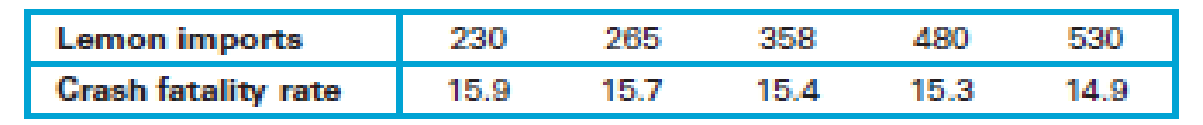
- 23. Lemons and Car Crashes. Listed below are annual data for various years. The data are weights (metric tons) of lemons imported from Mexico and U.S. car crash fatality rates per 100,000 population [based on data from “The Trouble with QSAR (or How I Learned to Stop Worrying and Embrace Fallacy)” by Stephen Johnson, Journal of Chemical Information and Modeling, Vol. 48, No. 1].
Expert Solution & Answer
Want to see the full answer?
Check out a sample textbook solution
Students have asked these similar questions
Business
3. Bayesian Inference – Updating Beliefs
A medical test for a rare disease has the following characteristics:
Sensitivity (true positive rate): 99%
Specificity (true negative rate): 98%
The disease occurs in 0.5% of the population.
A patient receives a positive test result.
Questions:
a) Define the relevant events and use Bayes’ Theorem to compute the probability that the patient actually has the disease.b) Explain why the result might seem counterintuitive, despite the high sensitivity and specificity.c) Discuss how prior probabilities influence posterior beliefs in Bayesian inference.d) Suppose a second, independent test with the same accuracy is conducted and is also positive. Update the probability that the patient has the disease.
4. Linear Regression - Model Assumptions and Interpretation
A real estate analyst is studying how house prices (Y) are related to house size in square feet (X). A simple
linear regression model is proposed:
The analyst fits the model and obtains:
•
Ŷ50,000+150X
YBoB₁X + €
•
R² = 0.76
• Residuals show a fan-shaped pattern when plotted against fitted values.
Questions:
a) Interpret the slope coefficient in context.
b) Explain what the R² value tells us about the model's performance.
c) Based on the residual pattern, what regression assumption is likely violated? What might be the
consequence?
d) Suggest at least two remedies to improve the model, based on the residual analysis.
Chapter 7 Solutions
Statistical Reasoning for Everyday Life (5th Edition)
Ch. 7.1 - Correlation. What is a correlation? Give three...Ch. 7.1 - Scatterplot. What is a scatterplot, and how is one...Ch. 7.1 - Types of Correlation. Define and distinguish...Ch. 7.1 - Correlation Coefficient. What does the correlation...Ch. 7.1 - Does It Make Sense? For Exercises 58, determine...Ch. 7.1 - Does It Make Sense? For Exercises 58, determine...Ch. 7.1 - Does It Make Sense? For Exercises 58, determine...Ch. 7.1 - Does It Make Sense? For Exercises 58, determine...Ch. 7.1 - Correlation. Exercises 916 list pairs of...Ch. 7.1 - Correlation. Exercises 916 list pairs of...
Ch. 7.1 - Correlation. Exercises 916 list pairs of...Ch. 7.1 - Correlation. Exercises 916 list pairs of...Ch. 7.1 - Correlation. Exercises 916 list pairs of...Ch. 7.1 - Correlation. Exercises 916 list pairs of...Ch. 7.1 - Correlation. Exercises 916 list pairs of...Ch. 7.1 - Correlation. Exercises 916 list pairs of...Ch. 7.1 - Crickets and Temperature. One classic example of a...Ch. 7.1 - Two-Day Forecast. Figure 7.8 shows a scatterplot...Ch. 7.1 - Properties of the Correlation Coefficient. For...Ch. 7.1 - Properties of the Correlation Coefficient. For...Ch. 7.1 - Properties of the Correlation Coefficient. For...Ch. 7.1 - Properties of the Correlation Coefficient. For...Ch. 7.1 - Scatterplot and Correlation. In Exercises 2330,...Ch. 7.1 - Scatterplot and Correlation. In Exercises 2330,...Ch. 7.1 - Scatterplot and Correlation. In Exercises 2330,...Ch. 7.1 - Prob. 26ECh. 7.1 - Scatterplot and Correlation. In Exercises 2330,...Ch. 7.1 - Scatterplot and Correlation. In Exercises 2330,...Ch. 7.1 - Scatterplot and Correlation. In Exercises 2330,...Ch. 7.1 - Scatterplot and Correlation. In Exercises 2330,...Ch. 7.1 - Your Own Positive Correlations. Give examples of...Ch. 7.1 - Your Own Negative Correlations. Give examples of...Ch. 7.2 - Outliers. Briefly explain how an outlier can make...Ch. 7.2 - Grouped Data. Briefly explain how data that...Ch. 7.2 - Explanations for Correlation. What are the three...Ch. 7.2 - Prob. 4ECh. 7.2 - Does It Make Sense? For Exercises 58, determine...Ch. 7.2 - Does It Make Sense? For Exercises 58, determine...Ch. 7.2 - Does It Make Sense? For Exercises 58, determine...Ch. 7.2 - Does It Make Sense? For Exercises 58, determine...Ch. 7.2 - Correlation and Causality. Exercises 916 present...Ch. 7.2 - Correlation and Causality. Exercises 916 present...Ch. 7.2 - Correlation and Causality. Exercises 916 present...Ch. 7.2 - Correlation and Causality. Exercises 916 present...Ch. 7.2 - Correlation and Causality. Exercises 916 present...Ch. 7.2 - Correlation and Causality. Exercises 916 present...Ch. 7.2 - Correlation and Causality. Exercises 916 present...Ch. 7.2 - Correlation and Causality. Exercises 916 present...Ch. 7.2 - Outlier Effects. Consider the scatterplot in...Ch. 7.2 - Outlier Effects. Consider the scatterplot in...Ch. 7.2 - Footprint and Height. The following table lists...Ch. 7.2 - January and July High Temperatures. The following...Ch. 7.2 - Birth and Death Rates. Figure 7.17 shows the birth...Ch. 7.2 - Penny Weight and Date. The scatterplot in Figure...Ch. 7.3 - Best-Fit Line. What is a best-fit line? How is a...Ch. 7.3 - Prob. 2ECh. 7.3 - Interpreting r2. What does the square of the...Ch. 7.3 - Prob. 4ECh. 7.3 - Prob. 5ECh. 7.3 - Does It Make Sense? For Exercises 58, determine...Ch. 7.3 - Does It Make Sense? For Exercises 58, determine...Ch. 7.3 - Does It Make Sense? For Exercises 58, determine...Ch. 7.3 - Best-Fit Lines. Exercises 916 refer to tables in...Ch. 7.3 - Best-Fit Lines. Exercises 916 refer to tables in...Ch. 7.3 - Prob. 11ECh. 7.3 - Best-Fit Lines. Exercises 916 refer to tables in...Ch. 7.3 - Best-Fit Lines. Exercises 916 refer to tables in...Ch. 7.3 - Best-Fit Lines. Exercises 916 refer to tables in...Ch. 7.3 - Prob. 15ECh. 7.3 - Prob. 16ECh. 7.4 - Correlation and Causality. What is the difference...Ch. 7.4 - Prob. 2ECh. 7.4 - Establishing Causality. Briefly state in your own...Ch. 7.4 - Confidence in Causality. Describe three levels of...Ch. 7.4 - Prob. 5ECh. 7.4 - Does It Make Sense? For Exercises 58, determine...Ch. 7.4 - Does It Make Sense? For Exercises 58, determine...Ch. 7.4 - Does It Make Sense? For Exercises 58, determine...Ch. 7.4 - Physical Models. For Exercises 912, determine...Ch. 7.4 - Physical Models. For Exercises 912, determine...Ch. 7.4 - Physical Models. For Exercises 912, determine...Ch. 7.4 - Physical Models. For Exercises 912, determine...Ch. 7.4 - Altitude and Health. When some people climb to...Ch. 7.4 - Smoking and Lung Cancer. There is a strong...Ch. 7.4 - Other Lung Cancer Causes. Several things besides...Ch. 7.4 - Longevity of Orchestra Conductors. A famous study...Ch. 7.4 - Older Moms. A study reported in Nature claims that...Ch. 7.4 - High-Voltage Power Lines. Suppose that people...Ch. 7.4 - Gun Control. Those who favor gun control often...Ch. 7.4 - Vasectomies and Prostate Cancer. The article Does...Ch. 7 - Pizza and the Subway. For Exercises 16, refer to...Ch. 7 - Pizza and the Subway. For Exercises 16, refer to...Ch. 7 - Pizza and the Subway. For Exercises 16, refer to...Ch. 7 - Pizza and the Subway. For Exercises 16, refer to...Ch. 7 - Pizza and the Subway. For Exercises 16, refer to...Ch. 7 - Pizza and the Subway. For Exercises 16, refer to...Ch. 7 - For 10 pairs of sample data values, the...Ch. 7 - In a study involving randomly selected subjects,...Ch. 7 - A researcher collects paired sample data values...Ch. 7 - Estimate the value of the linear correlation...Ch. 7 - Fill in the blanks: Every possible correlation...Ch. 7 - Which of the following are likely to have a...Ch. 7 - For a collection of 50 pairs of sample data...Ch. 7 - Estimate the correlation coefficient for the data...Ch. 7 - Refer again to the scatterplot in Figure 7.24....Ch. 7 - Fill in the blank: If r = 0.900, then _____ % of...Ch. 7 - In Exercises 710, determine whether the given...Ch. 7 - Prob. 8CQCh. 7 - Prob. 9CQCh. 7 - Prob. 10CQ
Knowledge Booster


Learn more about
Need a deep-dive on the concept behind this application? Look no further. Learn more about this topic, statistics and related others by exploring similar questions and additional content below.Similar questions
- 5. Probability Distributions – Continuous Random Variables A factory machine produces metal rods whose lengths (in cm) follow a continuous uniform distribution on the interval [98, 102]. Questions: a) Define the probability density function (PDF) of the rod length.b) Calculate the probability that a randomly selected rod is shorter than 99 cm.c) Determine the expected value and variance of rod lengths.d) If a sample of 25 rods is selected, what is the probability that their average length is between 99.5 cm and 100.5 cm? Justify your answer using the appropriate distribution.arrow_forward2. Hypothesis Testing - Two Sample Means A nutritionist is investigating the effect of two different diet programs, A and B, on weight loss. Two independent samples of adults were randomly assigned to each diet for 12 weeks. The weight losses (in kg) are normally distributed. Sample A: n = 35, 4.8, s = 1.2 Sample B: n=40, 4.3, 8 = 1.0 Questions: a) State the null and alternative hypotheses to test whether there is a significant difference in mean weight loss between the two diet programs. b) Perform a hypothesis test at the 5% significance level and interpret the result. c) Compute a 95% confidence interval for the difference in means and interpret it. d) Discuss assumptions of this test and explain how violations of these assumptions could impact the results.arrow_forward1. Sampling Distribution and the Central Limit Theorem A company produces batteries with a mean lifetime of 300 hours and a standard deviation of 50 hours. The lifetimes are not normally distributed—they are right-skewed due to some batteries lasting unusually long. Suppose a quality control analyst selects a random sample of 64 batteries from a large production batch. Questions: a) Explain whether the distribution of sample means will be approximately normal. Justify your answer using the Central Limit Theorem. b) Compute the mean and standard deviation of the sampling distribution of the sample mean. c) What is the probability that the sample mean lifetime of the 64 batteries exceeds 310 hours? d) Discuss how the sample size affects the shape and variability of the sampling distribution.arrow_forward
- A biologist is investigating the effect of potential plant hormones by treating 20 stem segments. At the end of the observation period he computes the following length averages: Compound X = 1.18 Compound Y = 1.17 Based on these mean values he concludes that there are no treatment differences. 1) Are you satisfied with his conclusion? Why or why not? 2) If he asked you for help in analyzing these data, what statistical method would you suggest that he use to come to a meaningful conclusion about his data and why? 3) Are there any other questions you would ask him regarding his experiment, data collection, and analysis methods?arrow_forwardBusinessarrow_forwardWhat is the solution and answer to question?arrow_forward
- To: [Boss's Name] From: Nathaniel D Sain Date: 4/5/2025 Subject: Decision Analysis for Business Scenario Introduction to the Business Scenario Our delivery services business has been experiencing steady growth, leading to an increased demand for faster and more efficient deliveries. To meet this demand, we must decide on the best strategy to expand our fleet. The three possible alternatives under consideration are purchasing new delivery vehicles, leasing vehicles, or partnering with third-party drivers. The decision must account for various external factors, including fuel price fluctuations, demand stability, and competition growth, which we categorize as the states of nature. Each alternative presents unique advantages and challenges, and our goal is to select the most viable option using a structured decision-making approach. Alternatives and States of Nature The three alternatives for fleet expansion were chosen based on their cost implications, operational efficiency, and…arrow_forwardBusinessarrow_forwardWhy researchers are interested in describing measures of the center and measures of variation of a data set?arrow_forward
- WHAT IS THE SOLUTION?arrow_forwardThe following ordered data list shows the data speeds for cell phones used by a telephone company at an airport: A. Calculate the Measures of Central Tendency from the ungrouped data list. B. Group the data in an appropriate frequency table. C. Calculate the Measures of Central Tendency using the table in point B. 0.8 1.4 1.8 1.9 3.2 3.6 4.5 4.5 4.6 6.2 6.5 7.7 7.9 9.9 10.2 10.3 10.9 11.1 11.1 11.6 11.8 12.0 13.1 13.5 13.7 14.1 14.2 14.7 15.0 15.1 15.5 15.8 16.0 17.5 18.2 20.2 21.1 21.5 22.2 22.4 23.1 24.5 25.7 28.5 34.6 38.5 43.0 55.6 71.3 77.8arrow_forwardII Consider the following data matrix X: X1 X2 0.5 0.4 0.2 0.5 0.5 0.5 10.3 10 10.1 10.4 10.1 10.5 What will the resulting clusters be when using the k-Means method with k = 2. In your own words, explain why this result is indeed expected, i.e. why this clustering minimises the ESS map.arrow_forward
arrow_back_ios
SEE MORE QUESTIONS
arrow_forward_ios
Recommended textbooks for you
 Glencoe Algebra 1, Student Edition, 9780079039897...AlgebraISBN:9780079039897Author:CarterPublisher:McGraw Hill
 Big Ideas Math A Bridge To Success Algebra 1: Stu...AlgebraISBN:9781680331141Author:HOUGHTON MIFFLIN HARCOURTPublisher:Houghton Mifflin Harcourt
 Holt Mcdougal Larson Pre-algebra: Student Edition...AlgebraISBN:9780547587776Author:HOLT MCDOUGALPublisher:HOLT MCDOUGAL
Glencoe Algebra 1, Student Edition, 9780079039897...
Algebra
ISBN:9780079039897
Author:Carter
Publisher:McGraw Hill
Big Ideas Math A Bridge To Success Algebra 1: Stu...
Algebra
ISBN:9781680331141
Author:HOUGHTON MIFFLIN HARCOURT
Publisher:Houghton Mifflin Harcourt
Holt Mcdougal Larson Pre-algebra: Student Edition...
Algebra
ISBN:9780547587776
Author:HOLT MCDOUGAL
Publisher:HOLT MCDOUGAL
Correlation Vs Regression: Difference Between them with definition & Comparison Chart; Author: Key Differences;https://www.youtube.com/watch?v=Ou2QGSJVd0U;License: Standard YouTube License, CC-BY
Correlation and Regression: Concepts with Illustrative examples; Author: LEARN & APPLY : Lean and Six Sigma;https://www.youtube.com/watch?v=xTpHD5WLuoA;License: Standard YouTube License, CC-BY