Statistical Reasoning for Everyday Life (5th Edition)
5th Edition
ISBN: 9780134494043
Author: Jeff Bennett, William L. Briggs, Mario F. Triola
Publisher: PEARSON
expand_more
expand_more
format_list_bulleted
Videos
Textbook Question
Chapter 7, Problem 4CRE
Pizza and the Subway. For Exercises 1–6, refer to the following table that lists the cost (in dollars) of a slice of pizza in New York City and the subway fare in the same year.
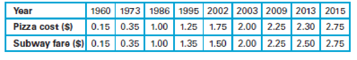
4. Find or estimate the value of r2. What does that value tell us?
Expert Solution & Answer
Want to see the full answer?
Check out a sample textbook solution
Students have asked these similar questions
310015
K
Question 9,
5.2.28-T
Part 1 of 4
HW Score:
85.96%, 49 of
57 points
Points: 1
Save
of 6
Based on a poll, among adults who regret getting tattoos, 28%
say that they were too young when they got their tattoos.
Assume that six adults who regret getting tattoos are
randomly selected, and find the indicated probability. Complete
parts (a) through (d) below.
a. Find the probability that none of the selected adults say that
they were too young to get tattoos.
0.0520 (Round to four decimal places as needed.)
Clear all
Final check
Feb 7 12:47 US O
how could the bar graph have been organized differently to make it easier to compare opinion changes within political parties
Draw a picture of a normal distribution with
mean 70 and standard deviation 5.
Chapter 7 Solutions
Statistical Reasoning for Everyday Life (5th Edition)
Ch. 7.1 - Correlation. What is a correlation? Give three...Ch. 7.1 - Scatterplot. What is a scatterplot, and how is one...Ch. 7.1 - Types of Correlation. Define and distinguish...Ch. 7.1 - Correlation Coefficient. What does the correlation...Ch. 7.1 - Does It Make Sense? For Exercises 58, determine...Ch. 7.1 - Does It Make Sense? For Exercises 58, determine...Ch. 7.1 - Does It Make Sense? For Exercises 58, determine...Ch. 7.1 - Does It Make Sense? For Exercises 58, determine...Ch. 7.1 - Correlation. Exercises 916 list pairs of...Ch. 7.1 - Correlation. Exercises 916 list pairs of...
Ch. 7.1 - Correlation. Exercises 916 list pairs of...Ch. 7.1 - Correlation. Exercises 916 list pairs of...Ch. 7.1 - Correlation. Exercises 916 list pairs of...Ch. 7.1 - Correlation. Exercises 916 list pairs of...Ch. 7.1 - Correlation. Exercises 916 list pairs of...Ch. 7.1 - Correlation. Exercises 916 list pairs of...Ch. 7.1 - Crickets and Temperature. One classic example of a...Ch. 7.1 - Two-Day Forecast. Figure 7.8 shows a scatterplot...Ch. 7.1 - Properties of the Correlation Coefficient. For...Ch. 7.1 - Properties of the Correlation Coefficient. For...Ch. 7.1 - Properties of the Correlation Coefficient. For...Ch. 7.1 - Properties of the Correlation Coefficient. For...Ch. 7.1 - Scatterplot and Correlation. In Exercises 2330,...Ch. 7.1 - Scatterplot and Correlation. In Exercises 2330,...Ch. 7.1 - Scatterplot and Correlation. In Exercises 2330,...Ch. 7.1 - Prob. 26ECh. 7.1 - Scatterplot and Correlation. In Exercises 2330,...Ch. 7.1 - Scatterplot and Correlation. In Exercises 2330,...Ch. 7.1 - Scatterplot and Correlation. In Exercises 2330,...Ch. 7.1 - Scatterplot and Correlation. In Exercises 2330,...Ch. 7.1 - Your Own Positive Correlations. Give examples of...Ch. 7.1 - Your Own Negative Correlations. Give examples of...Ch. 7.2 - Outliers. Briefly explain how an outlier can make...Ch. 7.2 - Grouped Data. Briefly explain how data that...Ch. 7.2 - Explanations for Correlation. What are the three...Ch. 7.2 - Prob. 4ECh. 7.2 - Does It Make Sense? For Exercises 58, determine...Ch. 7.2 - Does It Make Sense? For Exercises 58, determine...Ch. 7.2 - Does It Make Sense? For Exercises 58, determine...Ch. 7.2 - Does It Make Sense? For Exercises 58, determine...Ch. 7.2 - Correlation and Causality. Exercises 916 present...Ch. 7.2 - Correlation and Causality. Exercises 916 present...Ch. 7.2 - Correlation and Causality. Exercises 916 present...Ch. 7.2 - Correlation and Causality. Exercises 916 present...Ch. 7.2 - Correlation and Causality. Exercises 916 present...Ch. 7.2 - Correlation and Causality. Exercises 916 present...Ch. 7.2 - Correlation and Causality. Exercises 916 present...Ch. 7.2 - Correlation and Causality. Exercises 916 present...Ch. 7.2 - Outlier Effects. Consider the scatterplot in...Ch. 7.2 - Outlier Effects. Consider the scatterplot in...Ch. 7.2 - Footprint and Height. The following table lists...Ch. 7.2 - January and July High Temperatures. The following...Ch. 7.2 - Birth and Death Rates. Figure 7.17 shows the birth...Ch. 7.2 - Penny Weight and Date. The scatterplot in Figure...Ch. 7.3 - Best-Fit Line. What is a best-fit line? How is a...Ch. 7.3 - Prob. 2ECh. 7.3 - Interpreting r2. What does the square of the...Ch. 7.3 - Prob. 4ECh. 7.3 - Prob. 5ECh. 7.3 - Does It Make Sense? For Exercises 58, determine...Ch. 7.3 - Does It Make Sense? For Exercises 58, determine...Ch. 7.3 - Does It Make Sense? For Exercises 58, determine...Ch. 7.3 - Best-Fit Lines. Exercises 916 refer to tables in...Ch. 7.3 - Best-Fit Lines. Exercises 916 refer to tables in...Ch. 7.3 - Prob. 11ECh. 7.3 - Best-Fit Lines. Exercises 916 refer to tables in...Ch. 7.3 - Best-Fit Lines. Exercises 916 refer to tables in...Ch. 7.3 - Best-Fit Lines. Exercises 916 refer to tables in...Ch. 7.3 - Prob. 15ECh. 7.3 - Prob. 16ECh. 7.4 - Correlation and Causality. What is the difference...Ch. 7.4 - Prob. 2ECh. 7.4 - Establishing Causality. Briefly state in your own...Ch. 7.4 - Confidence in Causality. Describe three levels of...Ch. 7.4 - Prob. 5ECh. 7.4 - Does It Make Sense? For Exercises 58, determine...Ch. 7.4 - Does It Make Sense? For Exercises 58, determine...Ch. 7.4 - Does It Make Sense? For Exercises 58, determine...Ch. 7.4 - Physical Models. For Exercises 912, determine...Ch. 7.4 - Physical Models. For Exercises 912, determine...Ch. 7.4 - Physical Models. For Exercises 912, determine...Ch. 7.4 - Physical Models. For Exercises 912, determine...Ch. 7.4 - Altitude and Health. When some people climb to...Ch. 7.4 - Smoking and Lung Cancer. There is a strong...Ch. 7.4 - Other Lung Cancer Causes. Several things besides...Ch. 7.4 - Longevity of Orchestra Conductors. A famous study...Ch. 7.4 - Older Moms. A study reported in Nature claims that...Ch. 7.4 - High-Voltage Power Lines. Suppose that people...Ch. 7.4 - Gun Control. Those who favor gun control often...Ch. 7.4 - Vasectomies and Prostate Cancer. The article Does...Ch. 7 - Pizza and the Subway. For Exercises 16, refer to...Ch. 7 - Pizza and the Subway. For Exercises 16, refer to...Ch. 7 - Pizza and the Subway. For Exercises 16, refer to...Ch. 7 - Pizza and the Subway. For Exercises 16, refer to...Ch. 7 - Pizza and the Subway. For Exercises 16, refer to...Ch. 7 - Pizza and the Subway. For Exercises 16, refer to...Ch. 7 - For 10 pairs of sample data values, the...Ch. 7 - In a study involving randomly selected subjects,...Ch. 7 - A researcher collects paired sample data values...Ch. 7 - Estimate the value of the linear correlation...Ch. 7 - Fill in the blanks: Every possible correlation...Ch. 7 - Which of the following are likely to have a...Ch. 7 - For a collection of 50 pairs of sample data...Ch. 7 - Estimate the correlation coefficient for the data...Ch. 7 - Refer again to the scatterplot in Figure 7.24....Ch. 7 - Fill in the blank: If r = 0.900, then _____ % of...Ch. 7 - In Exercises 710, determine whether the given...Ch. 7 - Prob. 8CQCh. 7 - Prob. 9CQCh. 7 - Prob. 10CQ
Knowledge Booster


Learn more about
Need a deep-dive on the concept behind this application? Look no further. Learn more about this topic, statistics and related others by exploring similar questions and additional content below.Similar questions
- What do you guess are the standard deviations of the two distributions in the previous example problem?arrow_forwardPlease answer the questionsarrow_forward30. An individual who has automobile insurance from a certain company is randomly selected. Let Y be the num- ber of moving violations for which the individual was cited during the last 3 years. The pmf of Y isy | 1 2 4 8 16p(y) | .05 .10 .35 .40 .10 a.Compute E(Y).b. Suppose an individual with Y violations incurs a surcharge of $100Y^2. Calculate the expected amount of the surcharge.arrow_forward
- 24. An insurance company offers its policyholders a num- ber of different premium payment options. For a ran- domly selected policyholder, let X = the number of months between successive payments. The cdf of X is as follows: F(x)=0.00 : x < 10.30 : 1≤x<30.40 : 3≤ x < 40.45 : 4≤ x <60.60 : 6≤ x < 121.00 : 12≤ x a. What is the pmf of X?b. Using just the cdf, compute P(3≤ X ≤6) and P(4≤ X).arrow_forward59. At a certain gas station, 40% of the customers use regular gas (A1), 35% use plus gas (A2), and 25% use premium (A3). Of those customers using regular gas, only 30% fill their tanks (event B). Of those customers using plus, 60% fill their tanks, whereas of those using premium, 50% fill their tanks.a. What is the probability that the next customer will request plus gas and fill the tank (A2 B)?b. What is the probability that the next customer fills the tank?c. If the next customer fills the tank, what is the probability that regular gas is requested? Plus? Premium?arrow_forward38. Possible values of X, the number of components in a system submitted for repair that must be replaced, are 1, 2, 3, and 4 with corresponding probabilities .15, .35, .35, and .15, respectively. a. Calculate E(X) and then E(5 - X).b. Would the repair facility be better off charging a flat fee of $75 or else the amount $[150/(5 - X)]? [Note: It is not generally true that E(c/Y) = c/E(Y).]arrow_forward
- 74. The proportions of blood phenotypes in the U.S. popula- tion are as follows:A B AB O .40 .11 .04 .45 Assuming that the phenotypes of two randomly selected individuals are independent of one another, what is the probability that both phenotypes are O? What is the probability that the phenotypes of two randomly selected individuals match?arrow_forward53. A certain shop repairs both audio and video compo- nents. Let A denote the event that the next component brought in for repair is an audio component, and let B be the event that the next component is a compact disc player (so the event B is contained in A). Suppose that P(A) = .6 and P(B) = .05. What is P(BA)?arrow_forward26. A certain system can experience three different types of defects. Let A;(i = 1,2,3) denote the event that the sys- tem has a defect of type i. Suppose thatP(A1) = .12 P(A) = .07 P(A) = .05P(A, U A2) = .13P(A, U A3) = .14P(A2 U A3) = .10P(A, A2 A3) = .011Rshelfa. What is the probability that the system does not havea type 1 defect?b. What is the probability that the system has both type 1 and type 2 defects?c. What is the probability that the system has both type 1 and type 2 defects but not a type 3 defect? d. What is the probability that the system has at most two of these defects?arrow_forward
- The following are suggested designs for group sequential studies. Using PROCSEQDESIGN, provide the following for the design O’Brien Fleming and Pocock.• The critical boundary values for each analysis of the data• The expected sample sizes at each interim analysisAssume the standardized Z score method for calculating boundaries.Investigators are evaluating the success rate of a novel drug for treating a certain type ofbacterial wound infection. Since no existing treatment exists, they have planned a one-armstudy. They wish to test whether the success rate of the drug is better than 50%, whichthey have defined as the null success rate. Preliminary testing has estimated the successrate of the drug at 55%. The investigators are eager to get the drug into production andwould like to plan for 9 interim analyses (10 analyzes in total) of the data. Assume thesignificance level is 5% and power is 90%.Besides, draw a combined boundary plot (OBF, POC, and HP)arrow_forwardPlease provide the solution for the attached image in detailed.arrow_forward20 km, because GISS Worksheet 10 Jesse runs a small business selling and delivering mealie meal to the spaza shops. He charges a fixed rate of R80, 00 for delivery and then R15, 50 for each packet of mealle meal he delivers. The table below helps him to calculate what to charge his customers. 10 20 30 40 50 Packets of mealie meal (m) Total costs in Rands 80 235 390 545 700 855 (c) 10.1. Define the following terms: 10.1.1. Independent Variables 10.1.2. Dependent Variables 10.2. 10.3. 10.4. 10.5. Determine the independent and dependent variables. Are the variables in this scenario discrete or continuous values? Explain What shape do you expect the graph to be? Why? Draw a graph on the graph provided to represent the information in the table above. TOTAL COST OF PACKETS OF MEALIE MEAL 900 800 700 600 COST (R) 500 400 300 200 100 0 10 20 30 40 60 NUMBER OF PACKETS OF MEALIE MEALarrow_forward
arrow_back_ios
SEE MORE QUESTIONS
arrow_forward_ios
Recommended textbooks for you
 Algebra: Structure And Method, Book 1AlgebraISBN:9780395977224Author:Richard G. Brown, Mary P. Dolciani, Robert H. Sorgenfrey, William L. ColePublisher:McDougal Littell
 Big Ideas Math A Bridge To Success Algebra 1: Stu...AlgebraISBN:9781680331141Author:HOUGHTON MIFFLIN HARCOURTPublisher:Houghton Mifflin Harcourt
Algebra: Structure And Method, Book 1
Algebra
ISBN:9780395977224
Author:Richard G. Brown, Mary P. Dolciani, Robert H. Sorgenfrey, William L. Cole
Publisher:McDougal Littell
Big Ideas Math A Bridge To Success Algebra 1: Stu...
Algebra
ISBN:9781680331141
Author:HOUGHTON MIFFLIN HARCOURT
Publisher:Houghton Mifflin Harcourt
Hypothesis Testing using Confidence Interval Approach; Author: BUM2413 Applied Statistics UMP;https://www.youtube.com/watch?v=Hq1l3e9pLyY;License: Standard YouTube License, CC-BY
Hypothesis Testing - Difference of Two Means - Student's -Distribution & Normal Distribution; Author: The Organic Chemistry Tutor;https://www.youtube.com/watch?v=UcZwyzwWU7o;License: Standard Youtube License