Chapter 6, Problem 6.1.3RE

a.

To determine

To find: The probability $P\left(0<z<2.07\right)$ using the standard normal distribution.

Answer to Problem 6.1.3RE

The probability using the standard normal distribution is $\underset{\_}{P\left(0<z<2.07\right)=0.4808}$.

Explanation of Solution

Given info:

The z values are 0 and 2.07.

Calculation:

Software procedure:

Step by step procedure to find the area under the normal curve between 0 and 2.06with the help of following instructions:

• Select Graph > Probability Distribution Plot > View Probability >OK.
• From Distribution, choose ‘Normal’ distribution.
• Enter the Mean as 0.0 and Standard deviation as 1.0.
• Choose the tab for Shaded Area, then X Value.
• Click the picture for Middle.
• Type in the smaller value 0 for X value1 and then the larger value 2.07 for the X value2.
• Click OK.

Output using the MINITAB software is given below:

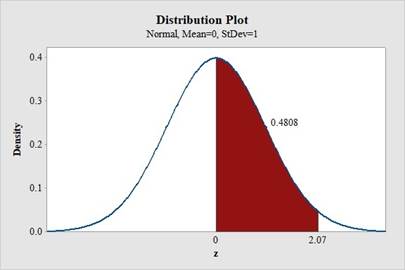
Therefore, $\underset{\_}{P\left(0<z<2.07\right)=0.4808}$

Conclusion:

The probability using the standard normal distribution is $\underset{\_}{P\left(0<z<2.07\right)=0.4808}$.

b.

To determine

To find: The probability $P\left(-1.83<z<0\right)$ using the standard normal distribution.

Answer to Problem 6.1.3RE

The probability using the standard normal distribution is $\underset{\_}{P\left(-1.83<z<0\right)=0.4664}$.

Explanation of Solution

Given info:

The z values are -1.83 and 0.

Calculation:

Software procedure:

Step by step procedure to find the area under the normal curve between 0 and 0.37 with the help of following instructions:

• Select Graph > Probability Distribution Plot > View Probability >OK.
• From Distribution, choose ‘Normal’ distribution.
• Enter the Mean as 0.0 and Standard deviation as 1.0.
• Choose the tab for Shaded Area, then X Value.
• Click the picture for Middle.
• Type in the smaller value -1.83 for X value1 and then the larger value 0 for the X value2.
• Click OK.

Output using the MINITAB software is given below:

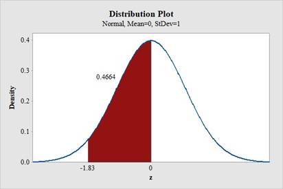
Therefore, $\underset{\_}{P\left(-1.83<z<0\right)=0.4664}$.

Conclusion:

The probability using the standard normal distribution is $\underset{\_}{P\left(-1.83<z<0\right)=0.4664}$.

c.

To determine

To find: The probability $P\left(-1.59<z<2.01\right)$ using the standard normal distribution.

Answer to Problem 6.1.3RE

The probability using the standard normal distribution is $\underset{\_}{P\left(-1.59<z<2.01\right)=0.9219}$.

Explanation of Solution

Given info:

The z values are -1.59 and 2.01.

Calculation:

Software procedure:

Step by step procedure to find the area under the normal curve between -1.59 and 2.01with the help of following instructions:

• Select Graph > Probability Distribution Plot > View Probability >OK.
• From Distribution, choose ‘Normal’ distribution.
• Enter the Mean as 0.0 and Standard deviation as 1.0.
• Choose the tab for Shaded Area, then X Value.
• Click the picture for Middle.
• Type in the smaller value -1.59 for X value1 and then the larger value 2.01 for the X value2.
• Click OK.

Output using the MINITAB software is given below:

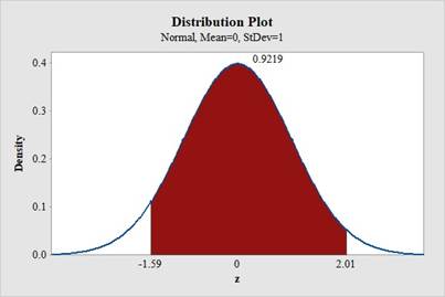
Therefore, $\underset{\_}{P\left(-1.59<z<2.01\right)=0.9219}$.

Conclusion:

The probability using the standard normal distribution is $\underset{\_}{P\left(-1.59<z<2.01\right)=0.9219}$.

d.

To determine

To find: The probability $P\left(1.33<z<1.88\right)$ using the standard normal distribution.

Answer to Problem 6.1.3RE

The probability using the standard normal distribution is $\underset{\_}{P\left(1.33<z<1.88\right)=0.06171}$.

Explanation of Solution

Given info:

The z values are 1.33 and 1.88.

Calculation:

Software procedure:

Step by step procedure to; find the area under the normal curve between 1.33 and 1.88with the help of following instructions:

• Select Graph > Probability Distribution Plot > View Probability >OK.
• From Distribution, choose ‘Normal’ distribution.
• Enter the Mean as 0.0 and Standard deviation as 1.0.
• Choose the tab for Shaded Area, then X Value.
• Click the picture for Middle.
• Type in the smaller value 1.33 for X value1 and then the larger value 1.88 for the X value2.
• Click OK.

Output using the MINITAB software is given below:

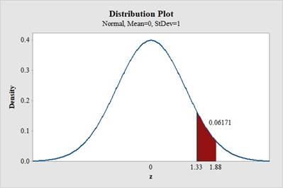
Therefore, $\underset{\_}{P\left(1.33<z<1.88\right)=0.06171}$.

Conclusion:

The probability using the standard normal distribution is $\underset{\_}{P\left(1.33<z<1.88\right)=0.06171}$.

e.

To determine

To find: The probability $P\left(-2.56<z<0.37\right)$ using the standard normal distribution.

Answer to Problem 6.1.3RE

The probability using the standard normal distribution is $\underset{\_}{P\left(-2.56<z<0.37\right)=0.6391}$.

Explanation of Solution

Given info:

The z values are -2.56 and 0.37.

Calculation:

Software procedure:

Step by step procedure to; find the area under the normal curve between -2.56 and 0.37 with the help of following instructions:

• Select Graph > Probability Distribution Plot > View Probability >OK.
• From Distribution, choose ‘Normal’ distribution.
• Enter the Mean as 0.0 and Standard deviation as 1.0.
• Choose the tab for Shaded Area, then X Value.
• Click the picture for Middle.
• Type in the smaller value −2.56 for X value1 and then the larger value 0.37 for the X value2.
• Click OK.

Output using the MINITAB software is given below:

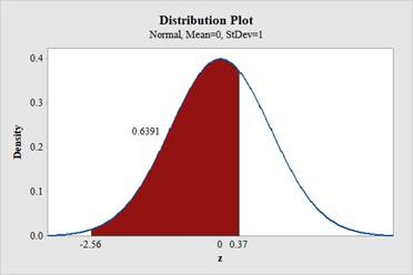
Therefore, $\underset{\_}{P\left(-2.56<z<0.37\right)=0.6391}$.

Conclusion:

The probability using the standard normal distribution is $\underset{\_}{P\left(-2.56<z<0.37\right)=0.6391}$.