Chapter 6, Problem 18CQ

Find the area under the standard normal distribution for each.

a. Between 0 and 1.50

b. Between 0 and −1.25

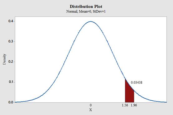
c. Between 1.56 and 1.96

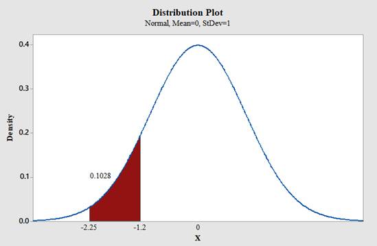
d. Between −1.20 and −2.25

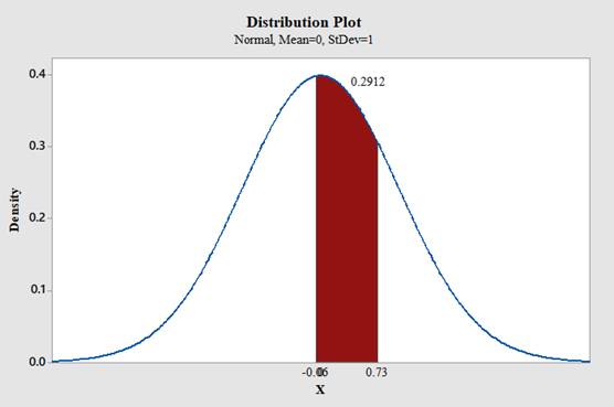
e. Between −0.06 and 0.73

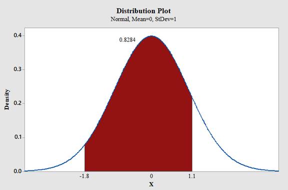
f. Between 1.10 and −1.80

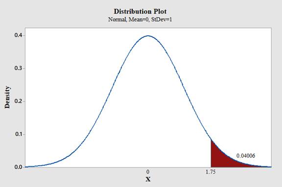
g. To the right of z = 1.75

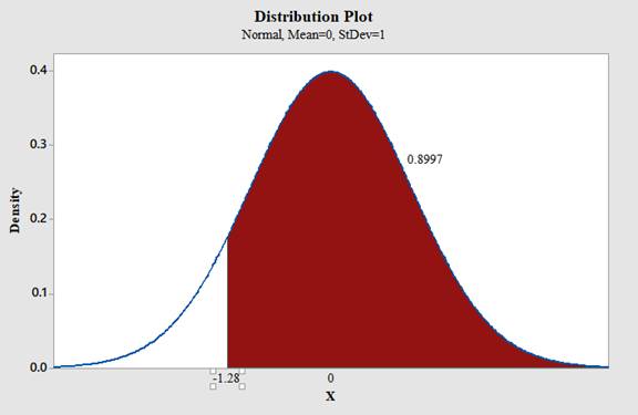
h. To the right of z = −1.28

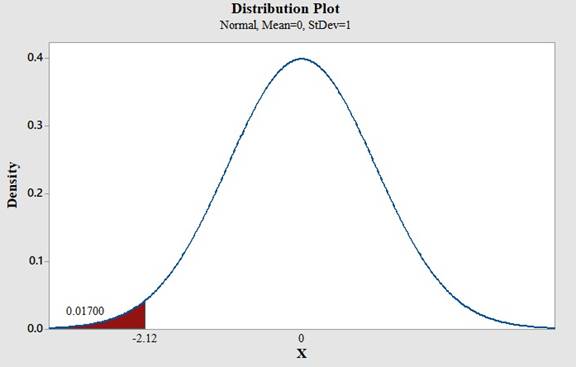
i. To the left of z = −2.12

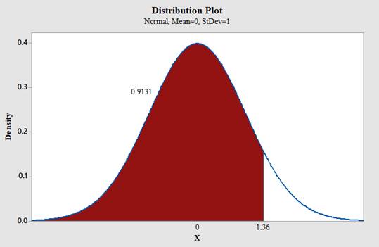
j. To the left of z = 1.36

To determine

To find: The area under the standard normal distribution curve for $z$ lies between 0 and 1.50. That is, $P\left(0<z<1.50\right).$

Answer to Problem 18CQ

The area under the standard normal distribution curve for $z$ lies between 0 and 1.50 is 0.433.

Explanation of Solution

Calculation:

Software procedure:

Use Minitab; find the area under the normal curve between 0 and 1.50 with the help of following instructions:

• Choose Graph > Probability Distribution Plot choose View Probability> OK.
• From Distribution, choose ‘Normal’ distribution.
• Enter the Mean as 0.0 and Standard deviation as 1.0.
• Click the Shaded Area tab.
• Click the picture for Middle.
• Type in the smaller value 0 for X value1 and then the larger value 1.50 for the X value2.
• Click OK.

Output using the MINITAB software is given below:

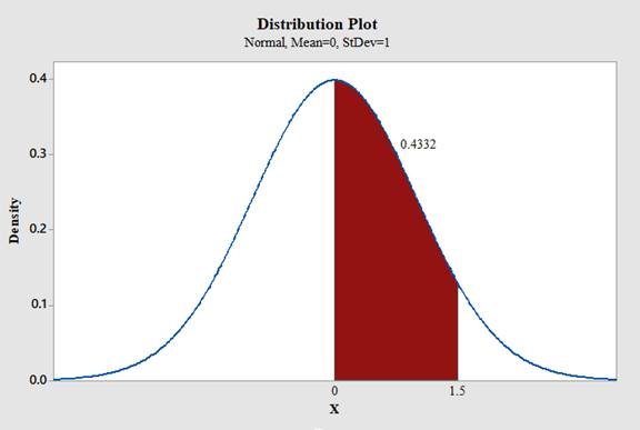
Therefore, $P\left(0<z<1.50\right)=\mathrm{0.433.}$

Conclusion:

The area under the standard normal distribution curve for $z$ lies between 0 and 1.50 is 0.433.

To determine

To find: The area under the standard normal distribution curve for $z$ lies between 0 and

 –1.25. That is, $P\left(-1.25<z<0\right).$

Answer to Problem 18CQ

The area under the standard normal distribution curve for $z$ lies between 0 and -1.25 is 0.394.

Explanation of Solution

Calculation:

Software procedure:

Use Minitab; find the area under the normal curve between 0 and -1.25 with the help of following instructions:

• Choose Graph > Probability Distribution Plot choose View Probability> OK.
• From Distribution, choose ‘Normal’ distribution.
• Enter the Mean as 0.0 and Standard deviation as 1.0.
• Click the Shaded Area tab.
• Click the picture for Middle.
• Type in the smaller value -1.25 for X value1 and then the larger value 0 for the X value2.
• Click OK.

Output using the MINITAB software is given below:

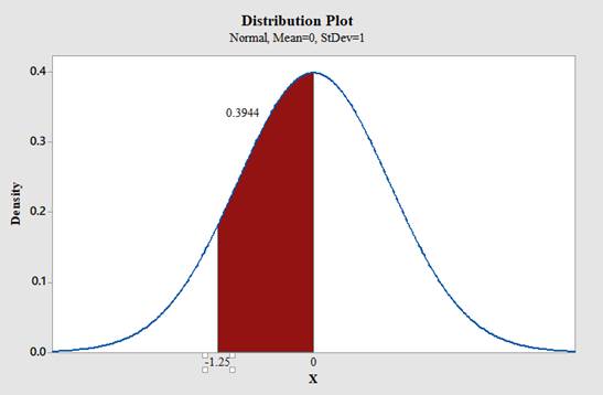
Therefore, $P\left(-1.25<z<0\right)=\mathrm{0.394.}$

Conclusion:

The area under the standard normal distribution curve for $z$ lies between 0 and -1.25 is 0.394.

To determine

To find: The area under the standard normal distribution curve for $z$ lies between 1.56 and 1.96. That is, $P\left(1.56<z<1.96\right).$

Answer to Problem 18CQ

The area under the standard normal distribution curve for $z$ lies between 1.56 and 1.96 is 0.0344.

Explanation of Solution

Calculation:

Software procedure:

Use Minitab; find the area under the normal curve between 1.56 and 1.96 with the help of following instructions:

• Choose Graph > Probability Distribution Plot choose View Probability> OK.
• From Distribution, choose ‘Normal’ distribution.
• Enter the Mean as 0.0 and Standard deviation as 1.0.
• Click the Shaded Area tab.
• Click the picture for Middle.
• Type in the smaller value 1.56 for X value1 and then the larger value 1.96 for the X value2.
• Click OK.

Output using the MINITAB software is given below:

.

Therefore, $P\left(1.56<z<1.96\right)=\mathrm{0.0344.}$

Conclusion:

The area under the standard normal distribution curve for $z$ lies between 1.56 and 1.96 is 0.0344.

To determine

To find: The area under the standard normal distribution curve for $z$ lies between -1.20 and –2.25. That is, $P\left(-2.25<z<-1.20\right).$

Answer to Problem 18CQ

The area under the standard normal distribution curve for $z$ lies between -1.20 and -2.25 is 0.103.

Explanation of Solution

Calculation:

Software procedure:

Use Minitab; find the area under the normal curve between -1.20 and -2.25 with the help of following instructions:

• Choose Graph > Probability Distribution Plot choose View Probability> OK.
• From Distribution, choose ‘Normal’ distribution.
• Enter the Mean as 0.0 and Standard deviation as 1.0.
• Click the Shaded Area tab.
• Click the picture for Middle.
• Type in the smaller value -2.25 for X value1 and then the larger value -1.20 for the X value2.
• Click OK.

Output using the MINITAB software is given below:

Therefore, $P\left(-2.25<z<-1.20\right)=0.103$.

Conclusion:

The area under the standard normal distribution curve for $z$ lies between -1.20 and -2.25 is 0.103.

To determine

To find: The area under the standard normal distribution curve for $z$ lies between -0.06 and 0.73. That is, $P\left(-0.06<z<0.73\right).$

Answer to Problem 18CQ

The area under the standard normal distribution curve for $z$ lies between -0.06 and 0.73 is 0.291.

Explanation of Solution

Calculation:

Software procedure:

Use Minitab; find the area under the normal curve between -0.06 and 0.73 with the help of following instructions:

• Choose Graph > Probability Distribution Plot choose View Probability> OK.
• From Distribution, choose ‘Normal’ distribution.
• Enter the Mean as 0.0 and Standard deviation as 1.0.
• Click the Shaded Area tab.
• Click the picture for Middle.
• Type in the smaller value -0.06 for X value1 and then the larger value 0.73 for the X value2.
• Click OK.

Output using the MINITAB software is given below:

.

Therefore, $P\left(-0.06<z<0.73\right)=0.291$

Conclusion:

The area under the standard normal distribution curve for $z$ lies between -0.06 and 0.73 is 0.291.

To determine

To find: The area under the standard normal distribution curve for $z$ lies between 1.10 and -1.80. That is, $P\left(-1.80<z<1.10\right).$

Answer to Problem 18CQ

The area under the standard normal distribution curve for $z$ lies between 1.10 and -1.80 is 0.828.

Explanation of Solution

Calculation:

Software procedure:

Use Minitab; find the area under the normal curve between 1.10 and -1.80 with the help of following instructions:

• Choose Graph > Probability Distribution Plot choose View Probability> OK.
• From Distribution, choose ‘Normal’ distribution.
• Enter the Mean as 0.0 and Standard deviation as 1.0.
• Click the Shaded Area tab.
• Click the picture for Middle.
• Type in the smaller value -1.80 for X value1 and then the larger value 1.10 for the X value2.
• Click OK.

Output using the MINITAB software is given below:

Therefore, $P\left(-1.80<z<1.10\right)=\mathrm{0.828.}$

Conclusion:

The area under the standard normal distribution curve for $z$ lies between 1.10 and -1.80 is 0.828.

To determine

To find: The area under the standard normal curve to the right of $z=\mathrm{1.75.}$

Answer to Problem 18CQ

The area under the standard normal curve to the right of $z=1.75$ is 0.0401.

Explanation of Solution

Calculation:

Software procedure:

Use Minitab; find the area under the normal curve to the right of 1.75 with the help of following instructions:

• Choose Graph > Probability Distribution Plot choose View Probability> OK.
• From Distribution, choose ‘Normal’ distribution.
• Enter the Mean as 0.0 and Standard deviation as 1.0.
• Click the Shaded Area tab.
• Click the picture for Right Trail.
• Type in the Z value of 1.75 and click OK.

Output using the MINITAB software is given below:

Therefore, $P\left(z>1.75\right)=\mathrm{0.0401.}$

Conclusion:

The area under the standard normal curve to the right of $z=1.75$ is 0.0401.

To determine

To find: The area under the standard normal curve to the right of $z=-\mathrm{1.28.}$

Answer to Problem 18CQ

The area under the standard normal curve to the right of $z=-1.28$ is 0.8997.

Explanation of Solution

Calculation:

Software procedure:

Use Minitab; find the area under the normal curve to the right of -1.28 with the help of following instructions:

• Choose Graph > Probability Distribution Plot choose View Probability> OK.
• From Distribution, choose ‘Normal’ distribution.
• Enter the Mean as 0.0 and Standard deviation as 1.0.
• Click the Shaded Area tab.
• Click the picture for Right Trail.
• Type in the Z value of -1.28 and click OK.

Output using the MINITAB software is given below:

Therefore, $P\left(z>-1.28\right)=0.8997$

Conclusion:

The area under the standard normal curve to the right of $z=-1.28$ is 0.8997.

To determine

To find: The area under the standard normal curve to the left of $z=-\mathrm{2.12.}$

Answer to Problem 18CQ

The area under the standard normal curve to the left of $z=-2.12$ is 0.0170.

Explanation of Solution

Calculation:

Software procedure:

Use Minitab; find the area under the normal curve to the left of -2.12 with the help of following instructions:

• Choose Graph > Probability Distribution Plot choose View Probability> OK.
• From Distribution, choose ‘Normal’ distribution.
• Enter the Mean as 0.0 and Standard deviation as 1.0.
• Click the Shaded Area tab.
• Click the picture for Left Trail.
• Type in the Z value of -2.12 and click OK.

Output using the MINITAB software is given below:

Therefore, $P\left(z<-2.12\right)=\mathrm{0.0170.}$

Conclusion:

The area under the standard normal curve to the left of $z=-2.12$ is 0.0170.

To determine

To find: The area under the standard normal curve to the left of $z=\mathrm{1.36.}$

Answer to Problem 18CQ

The area under the standard normal curve to the left of $z=1.36$ is 0.913.

Explanation of Solution

Calculation:

Software procedure:

Use Minitab; find the area under the normal curve to the left of 1.36 with the help of following instructions:

• Choose Graph > Probability Distribution Plot choose View Probability> OK.
• From Distribution, choose ‘Normal’ distribution.
• Enter the Mean as 0.0 and Standard deviation as 1.0.
• Click the Shaded Area tab.
• Click the picture for Left Trail.
• Type in the Z value of 1.36 and click OK.

Output using the MINITAB software is given below:

Therefore, $P\left(z<1.36\right)=\mathrm{0.913.}$

Conclusion:

The area under the standard normal curve to the left of $z=1.36$ is 0.913.