
Concept explainers
Videos
a)
To explain which one is better summary of the percentage of White residents in the neighborhoods.
a)
Answer to Problem 36E
Explanation of Solution
Given:

The distribution is left skewed. Therefore, when the distribution is left skewed then the
b)
To explain which one is better summary of the spread.
b)
Answer to Problem 36E
IQR.
Explanation of Solution
Given:

The distribution is left skewed. Therefore, when the distribution is left skewed then the standard deviation is highly influenced by the outlier points. Hence, IQR would better summary statistics as it is more resistant to skewed effects.
c)
To find the percent of neighborhood within 1 standard deviation.
c)
Answer to Problem 36E
The 68% of the values are within 1 standard deviation of the mean.
Explanation of Solution
Given:

According to rule of 68-95-99.7, the 68% of the values are within 1 standard deviation of the mean.
d)
To find the actual percent of neighborhood within 1 standard deviation.
d)
Answer to Problem 36E
More than 80% of the values are within 1 standard deviation of the mean.
Explanation of Solution
Given:

Form Histogram, more than 80% of the neighborhoods have a white percentage greater than 61.33%. Therefore, about 80% of the data lies within 1 standard deviation from the mean.
e)
To explain discrepancy between part c and part d.
e)
Answer to Problem 36E
The assumptions of Normal model do not fit so there is discrepancy between part c and d.
Explanation of Solution
Given:
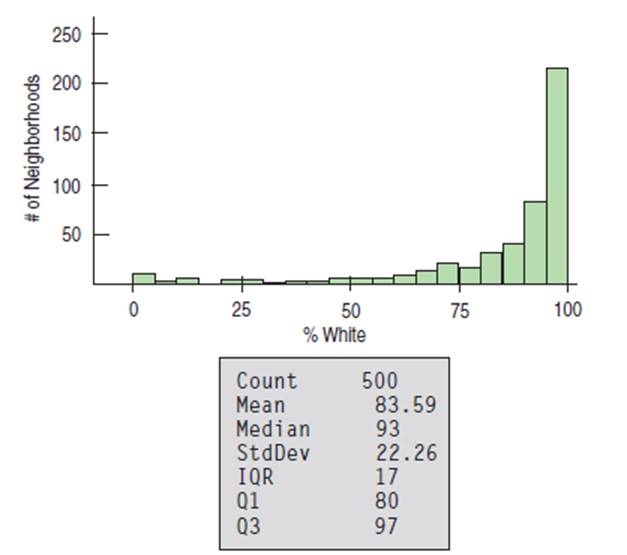
As we know, the distribution is left skewed and we can not use Normal model for this distribution. That’s why there is discrepancy between part c and d.
Chapter 6 Solutions
Stats: Modeling the World Nasta Edition Grades 9-12
Additional Math Textbook Solutions
A Problem Solving Approach To Mathematics For Elementary School Teachers (13th Edition)
Calculus: Early Transcendentals (2nd Edition)
University Calculus: Early Transcendentals (4th Edition)
Basic Business Statistics, Student Value Edition


- In a company with 80 employees, 60 earn $10.00 per hour and 20 earn $13.00 per hour. Is this average hourly wage considered representative?arrow_forwardThe following is a list of questions answered correctly on an exam. Calculate the Measures of Central Tendency from the ungrouped data list. NUMBER OF QUESTIONS ANSWERED CORRECTLY ON AN APTITUDE EXAM 112 72 69 97 107 73 92 76 86 73 126 128 118 127 124 82 104 132 134 83 92 108 96 100 92 115 76 91 102 81 95 141 81 80 106 84 119 113 98 75 68 98 115 106 95 100 85 94 106 119arrow_forwardThe following ordered data list shows the data speeds for cell phones used by a telephone company at an airport: A. Calculate the Measures of Central Tendency using the table in point B. B. Are there differences in the measurements obtained in A and C? Why (give at least one justified reason)? 0.8 1.4 1.8 1.9 3.2 3.6 4.5 4.5 4.6 6.2 6.5 7.7 7.9 9.9 10.2 10.3 10.9 11.1 11.1 11.6 11.8 12.0 13.1 13.5 13.7 14.1 14.2 14.7 15.0 15.1 15.5 15.8 16.0 17.5 18.2 20.2 21.1 21.5 22.2 22.4 23.1 24.5 25.7 28.5 34.6 38.5 43.0 55.6 71.3 77.8arrow_forward
- In a company with 80 employees, 60 earn $10.00 per hour and 20 earn $13.00 per hour. a) Determine the average hourly wage. b) In part a), is the same answer obtained if the 60 employees have an average wage of $10.00 per hour? Prove your answer.arrow_forwardThe following ordered data list shows the data speeds for cell phones used by a telephone company at an airport: A. Calculate the Measures of Central Tendency from the ungrouped data list. B. Group the data in an appropriate frequency table. 0.8 1.4 1.8 1.9 3.2 3.6 4.5 4.5 4.6 6.2 6.5 7.7 7.9 9.9 10.2 10.3 10.9 11.1 11.1 11.6 11.8 12.0 13.1 13.5 13.7 14.1 14.2 14.7 15.0 15.1 15.5 15.8 16.0 17.5 18.2 20.2 21.1 21.5 22.2 22.4 23.1 24.5 25.7 28.5 34.6 38.5 43.0 55.6 71.3 77.8arrow_forwardBusinessarrow_forward
- https://www.hawkeslearning.com/Statistics/dbs2/datasets.htmlarrow_forwardNC Current Students - North Ce X | NC Canvas Login Links - North ( X Final Exam Comprehensive x Cengage Learning x WASTAT - Final Exam - STAT → C webassign.net/web/Student/Assignment-Responses/submit?dep=36055360&tags=autosave#question3659890_9 Part (b) Draw a scatter plot of the ordered pairs. N Life Expectancy Life Expectancy 80 70 600 50 40 30 20 10 Year of 1950 1970 1990 2010 Birth O Life Expectancy Part (c) 800 70 60 50 40 30 20 10 1950 1970 1990 W ALT 林 $ # 4 R J7 Year of 2010 Birth F6 4+ 80 70 60 50 40 30 20 10 Year of 1950 1970 1990 2010 Birth Life Expectancy Ox 800 70 60 50 40 30 20 10 Year of 1950 1970 1990 2010 Birth hp P.B. KA & 7 80 % 5 H A B F10 711 N M K 744 PRT SC ALT CTRLarrow_forwardHarvard University California Institute of Technology Massachusetts Institute of Technology Stanford University Princeton University University of Cambridge University of Oxford University of California, Berkeley Imperial College London Yale University University of California, Los Angeles University of Chicago Johns Hopkins University Cornell University ETH Zurich University of Michigan University of Toronto Columbia University University of Pennsylvania Carnegie Mellon University University of Hong Kong University College London University of Washington Duke University Northwestern University University of Tokyo Georgia Institute of Technology Pohang University of Science and Technology University of California, Santa Barbara University of British Columbia University of North Carolina at Chapel Hill University of California, San Diego University of Illinois at Urbana-Champaign National University of Singapore McGill…arrow_forward
- Name Harvard University California Institute of Technology Massachusetts Institute of Technology Stanford University Princeton University University of Cambridge University of Oxford University of California, Berkeley Imperial College London Yale University University of California, Los Angeles University of Chicago Johns Hopkins University Cornell University ETH Zurich University of Michigan University of Toronto Columbia University University of Pennsylvania Carnegie Mellon University University of Hong Kong University College London University of Washington Duke University Northwestern University University of Tokyo Georgia Institute of Technology Pohang University of Science and Technology University of California, Santa Barbara University of British Columbia University of North Carolina at Chapel Hill University of California, San Diego University of Illinois at Urbana-Champaign National University of Singapore…arrow_forwardA company found that the daily sales revenue of its flagship product follows a normal distribution with a mean of $4500 and a standard deviation of $450. The company defines a "high-sales day" that is, any day with sales exceeding $4800. please provide a step by step on how to get the answers in excel Q: What percentage of days can the company expect to have "high-sales days" or sales greater than $4800? Q: What is the sales revenue threshold for the bottom 10% of days? (please note that 10% refers to the probability/area under bell curve towards the lower tail of bell curve) Provide answers in the yellow cellsarrow_forwardFind the critical value for a left-tailed test using the F distribution with a 0.025, degrees of freedom in the numerator=12, and degrees of freedom in the denominator = 50. A portion of the table of critical values of the F-distribution is provided. Click the icon to view the partial table of critical values of the F-distribution. What is the critical value? (Round to two decimal places as needed.)arrow_forward
 MATLAB: An Introduction with ApplicationsStatisticsISBN:9781119256830Author:Amos GilatPublisher:John Wiley & Sons Inc
 Probability and Statistics for Engineering and th...StatisticsISBN:9781305251809Author:Jay L. DevorePublisher:Cengage Learning
 Statistics for The Behavioral Sciences (MindTap C...StatisticsISBN:9781305504912Author:Frederick J Gravetter, Larry B. WallnauPublisher:Cengage Learning
 Elementary Statistics: Picturing the World (7th E...StatisticsISBN:9780134683416Author:Ron Larson, Betsy FarberPublisher:PEARSON
 The Basic Practice of StatisticsStatisticsISBN:9781319042578Author:David S. Moore, William I. Notz, Michael A. FlignerPublisher:W. H. Freeman
 Introduction to the Practice of StatisticsStatisticsISBN:9781319013387Author:David S. Moore, George P. McCabe, Bruce A. CraigPublisher:W. H. Freeman