Chapter 6, Problem 29E

a)

To determine

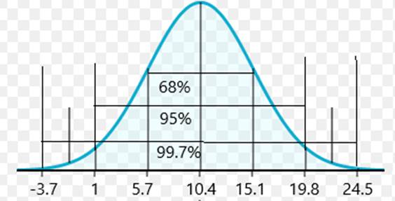
To draw the model which shows 68-95-99.7

Explanation of Solution

Given:

  $\mu$ = 10.4

  $\sigma$ = 4.7

Following is the model which shows 68-95-99.7:

  

b)

To determine

To explain what size to be expected that central 95% of all trees.

Answer to Problem 29E

An interval in which central 95% of trees to be found between 1 and 19.8

Explanation of Solution

Given:

  $\mu$ = 10.4

  $\sigma$ = 4.7

According to rule of 68-95-99.7, the 95% of the values are within 2 standard deviation of the mean.

Therefore,

  $\begin{array}{l}\mu -2\sigma =10.4-2\times 4.7=1\\ \mu +2\sigma =10.4+2\times 4.7=19.8\end{array}$

Hence, interval in which central 95% of trees to be found between 1 and 19.8

c)

To determine

To find the percentage of trees that should be less than 1 inch in diameter.

Answer to Problem 29E

The 2.5% of the trees are less than an inch in diameter.

Explanation of Solution

Given:

  $\mu$ = 10.4

  $\sigma$ = 4.7

According to rule of 68-95-99.7, the 95% of the values are within 2 standard deviation of the mean.

Therefore,

  $\begin{array}{l}\mu -2\sigma =10.4-2\times 4.7=1\\ \mu +2\sigma =10.4+2\times 4.7=19.8\end{array}$

That means, 1 inch is two standard deviations from the mean. According to rule, 95% of the data lies between 2 standard deviations from the mean. Since, total data is 100%, so 5% of the data is the more than 2 standard deviations from the mean. Therefore, as per symmetry, 2.5% is more than 2 standard deviations below the mean and 2.5% is more than 2 standard deviations above the mean.

Hence, approximately 2.5% of the trees are less than an inch in diameter.

d)

To determine

To find the percentage of trees that should be between 5.7 and 10.4 in diameter.

Answer to Problem 29E

The 32% of the trees are between 5.7 and 10.4 an inch in diameter.

Explanation of Solution

Given:

  $\mu$ = 10.4

  $\sigma$ = 4.7

According to rule of 68-95-99.7, the 68% of the values are within 1 standard deviation of the mean.

Therefore,

  $\mu -\sigma =10.4-4.7=5.7$

That means, 5.7 is one standard deviation below the mean.

Therefore, 100%-68% = 32% which is more than mean and less than 1 standard deviation of the mean. Therefore, 32% of the data lie between 5.7 and 10.4

e)

To determine

To find the percentage of trees that should be over 15 in diameter.

Answer to Problem 29E

The 2.5% of the trees should over 15 inches in diameter.

Explanation of Solution

Given:

  $\mu$ = 10.4

  $\sigma$ = 4.7

According to rule of 68-95-99.7, 15 is 2 standard deviation from the mean.

According to rule, 95% of the data lies between 2 standard deviations from the mean. Since, total data is 100%, so 5% of the data is the more than 2 standard deviations from the mean. Therefore, as per symmetry, 2.5% is more than 2 standard deviations below the mean and 2.5% is more than 2 standard deviations above the mean.

Hence, 2.5% of the trees should over 15 inches in diameter.