Chapter 5, Problem 78CR

An accurate assessment of oxygen consumption provides important information for determining energy expenditure requirements for physically demanding tasks. The paper “Oxygen Consumption During Fire Suppression: Error of Heart Rate Estimation” (Ergonomics [1991]: 1469–1474) reported on a study in which x = Oxygen consumption (in milliliters per kilogram per minute) during a treadmill test was determined for a sample of 10 firefighters. Then y = Oxygen consumption at a comparable heart rate was measured for each of the 10 individuals while they performed a fire-suppression simulation. This resulted in the following data and scatterplot:

1. a. Does the scatterplot suggest an approximate linear relationship?
2. b. The investigators fit a least-squares line. The resulting Minitab output is given in the following:

   The regression equation is firecon = 211. 4 + 1. 09 treadcon

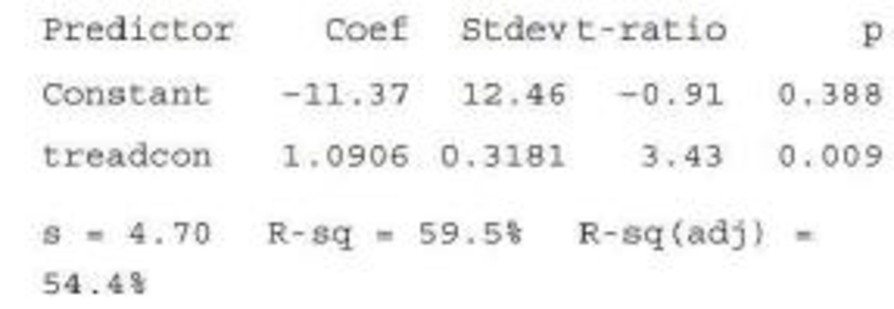
Predict fire-simulation consumption when treadmill consumption is 40.

1. c. How effectively does a straight line summarize the relationship?
2. d. Delete the first observation, (51.3, 49.3), and calculate the new equation of the least-squares line and the value of r². What do you conclude? (Hint: For the original data, Σx = 388.8, Σy = 310 .3, Σx² = 15,338.54, Σxy ＝ 12,306.58, and Σy² = 10,072.41.)

To determine

Discuss whether the scatterplot indicates an approximate linear relationship.

Answer to Problem 78CR

No, the scatterplot does not indicate an approximate linear relationship.

Explanation of Solution

The data relates the oxygen consumption (milliliters per kilogram per minute) of 10 firefighters during a fire-suppression simulation, y to that during a treadmill test, x. The scatterplot between the two variables is given.

Denote the estimated response variable as $\widehat{y}$.

A careful inspection of the given scatterplot shows that the points do not fall on a straight line. Rather, the points are scattered almost in a random manner, without showing any pattern in particular. However, there is one extreme point, which is far away from the remaining points. This extreme point appears to provide an impression that there might be a linear relationship between the two variables. Once this point is ignored, it is clear that no such relationship can be determined.

Thus, the scatterplot does not indicate an approximate linear relationship.

To determine

Predict the fire-simulation oxygen consumption, if the treadmill oxygen consumption is 40.

Answer to Problem 78CR

The fire-simulation oxygen consumption, when the treadmill oxygen consumption is 40 is 32.254 milliliters per kilogram per minute.

Explanation of Solution

Calculation:

The MINITAB output for the fitting of a least-squares regression line to the given data is given.

In the given output, the column of “Coef” gives the coefficients corresponding to the variables given in the column of “Predictor”. The term “Constant” under the column of ‘Predictor’ gives the intercept of the equation; the term “treadcon” denotes the oxygen consumption of during the treadmill test, x.

Using the values in the output, the equation of the least-squares regression line is $\widehat{y}=-11.37+1.0906x$.

For a treadmill oxygen consumption of 40 milliliters per kilogram per minute, $x=40$. Substitute this value in the above least-squares equation to predict the response variable:

$\begin{array}{c}\widehat{y}=-11.37+1.0906x\\ =-11.37+\left(1.0906\times 40\right)\\ =-11.37+43.624\\ =\mathrm{32.254.}\end{array}$

Thus, the fire-simulation oxygen consumption, when the treadmill oxygen consumption is 40 is 32.254 milliliters per kilogram per minute.

To determine

Explain the effectivity of the straight line to summarize the relationship between the variables.

Explanation of Solution

In the given output, the value of $r^2$ is reported as $\text{R-sq}=59.5\%$.

Now, $r^2$ is the percentage of variability in the response variable that can be explained by the regression model involving the given predictor variable.

Thus, it can be interpreted that the oxygen consumption during the treadmill test can predict about 59.5% of the variability in the oxygen consumption during the fire-suppression simulation.

This suggests that the straight line is moderately effective in summarizing the relationship between the variables.

To determine

Find the equation of the least-squares line and the value of $r^2$, after deleting the first observation, (51.3, 49.3).

Answer to Problem 78CR

The equation of the least-squares line after deleting the first observation, (51.3, 49.3) is $\underset{\_}{\widehat{y}=36.4175-0.1978x}$.

The value of $r^2$ after deleting the first observation, (51.3, 49.3) is 0.02.

Explanation of Solution

Calculation:

It is given that, for the original data set, ${\displaystyle \sum x}=388.8$, ${\displaystyle \sum y}=310.3$, ${\displaystyle \sum x^2}=15,338.54$, ${\displaystyle \sum xy}=12,306.58$ and ${\displaystyle \sum y^2}=10,072.41$. The first observation, (51.3, 49.3) is deleted. Thus, the new data set contains $n=9$ observations.

For the first observation, $x=51.3$, $y=49.3$. If this observation is deleted, the values of ${\displaystyle \sum x}$, ${\displaystyle \sum y}$, ${\displaystyle \sum x^2}$, ${\displaystyle \sum xy}$ and ${\displaystyle \sum y^2}$ change as follows:

$\begin{array}{c}{\displaystyle \sum x}=388.8-51.3\\ =\mathrm{337.5.}\end{array}$

$\begin{array}{c}{\displaystyle \sum y}=310.3-49.3\\ =261.\end{array}$

$\begin{array}{c}{\displaystyle \sum x^2}=15,338.54-{\left(51.3\right)}^2\\ =15,338.54-2,631.69\\ =12,\mathrm{706.85.}\end{array}$

$\begin{array}{c}{\displaystyle \sum xy}=12,306.58-\left(51.3\right)\cdot \left(49.3\right)\\ =12,306.58-2,529.09\\ =9,\mathrm{777.49.}\end{array}$

$\begin{array}{c}{\displaystyle \sum y^2}=10,072.41-{\left(49.3\right)}^2\\ =10,072.41-2,430.49\\ =7,\mathrm{641.92.}\end{array}$

Now, the lest-squares regression line is of the form: $\widehat{y}=a+bx$, where the intercept, $a=\overline{y}-b\overline{x}$ and the slope, $b=\frac{{\displaystyle \sum xy}-\frac{\left({\displaystyle \sum x}\right)\left({\displaystyle \sum y}\right)}{n}}{{\displaystyle \sum x^2}-\frac{{\left({\displaystyle \sum x}\right)}^2}{n}}$, with $\overline{y}$ denoting the mean of the response variable, y.

Using this formula and the values obtained above, b and a are respectively obtained as follows:

$\begin{array}{c}b=\frac{{\displaystyle \sum xy}-\frac{\left({\displaystyle \sum x}\right)\left({\displaystyle \sum y}\right)}{n}}{{\displaystyle \sum x^2}-\frac{{\left({\displaystyle \sum x}\right)}^2}{n}}\\ =\frac{9,777.49-\frac{\left(337.5\right)\left(261\right)}{9}}{12,706.85-\frac{{\left(337.5\right)}^2}{9}}\\ =\frac{9,777.49-9,787.5}{12,706.85-12,656.25}\\ =\frac{-10.01}{50.6}\\ \approx -\mathrm{0.1978.}\end{array}$

Now,

$\begin{array}{c}\overline{x}=\frac{1}{n}{\displaystyle \sum x}\\ =\frac{337.5}{9}\\ =\mathrm{37.5.}\end{array}$

$\begin{array}{c}\overline{y}=\frac{1}{n}{\displaystyle \sum y}\\ =\frac{261}{9}\\ =29.\end{array}$

Thus,

$\begin{array}{c}a=\overline{y}-b\overline{x}\\ =29-\left(-0.1978\right)\cdot \left(37.5\right)\\ =29+7.4175\\ =\mathrm{36.4175.}\end{array}$

Using the values of a and b obtained above, the equation of the least-squares line after deleting the first observation, (51.3, 49.3) is $\underset{\_}{\widehat{y}=36.4175-0.1978x}$.

Now, it is known that the slope for the least-squares regression of y on x, that is, b can be given by the formula: $b=r\frac{s_y}{s_x}$, where $s_x$ and $s_y$ are respectively the standard deviations of x and y. As a result, $r=b\frac{s_x}{s_y}$.

Now, it can be shown that:

$\begin{array}{c}{s}_x=\sqrt{\frac{{\displaystyle \sum {\left(x-\overline{x}\right)}^2}}{n-1}}\\ =\sqrt{\frac{{\displaystyle \sum x^2}-\frac{{\displaystyle \sum x}}{n}}{n-1}}.\end{array}$

Similarly,

$\begin{array}{c}{s}_y=\sqrt{\frac{{\displaystyle \sum {\left(y-\overline{y}\right)}^2}}{n-1}}\\ =\sqrt{\frac{{\displaystyle \sum y^2}-\frac{{\displaystyle \sum y}}{n}}{n-1}}.\end{array}$

Thus,

$\begin{array}{c}r=b\frac{s_x}{s_y}\\ =b\frac{\sqrt{\frac{{\displaystyle \sum x^2}-\frac{\left({\displaystyle \sum x}\right)}{n}}{n-1}}}{\sqrt{\frac{{\displaystyle \sum y^2}-\frac{\left({\displaystyle \sum y}\right)}{n}}{n-1}}}\\ =b\frac{\sqrt{{\displaystyle \sum x^2}-\frac{{\left({\displaystyle \sum x}\right)}^2}{n}}}{\sqrt{{\displaystyle \sum y^2}-\frac{{\left({\displaystyle \sum y}\right)}^2}{n}}}.\end{array}$

Using the values obtained above, the value of r can be calculated as follows:

$\begin{array}{c}r=b\frac{\sqrt{{\displaystyle \sum x^2}-\frac{{\left({\displaystyle \sum x}\right)}^2}{n}}}{\sqrt{{\displaystyle \sum y^2}-\frac{{\left({\displaystyle \sum y}\right)}^2}{n}}}\\ =\left(-0.1978\right)\frac{\sqrt{50.6}}{\sqrt{7,641.92-\frac{{\left(261\right)}^2}{9}}}\\ =\left(-0.1978\right)\frac{\sqrt{50.6}}{\sqrt{7,641.92-7,569}}\\ =\left(-0.1978\right)\frac{\sqrt{50.6}}{\sqrt{92.92}}\\ \approx -\mathrm{0.146.}\end{array}$

It is known that $r^2$ is simply the square of r. Thus,

$\begin{array}{c}{r}^2={\left(-0.146\right)}^2\\ \approx \mathrm{0.02.}\end{array}$

Hence, the value of $r^2$ after deleting the first observation, (51.3, 49.3) is 0.02.

Now, $r^2$ multiplied by 100, gives the percentage of variability in the response variable that can be explained by the regression model involving the given predictor variable.

Now,

$\begin{array}{c}100r^2=100\times 0.02\\ =2\%.\end{array}$

Thus, it can be interpreted that the oxygen consumption during the treadmill test can predict about 2% of the variability in the oxygen consumption during the fire-suppression simulation, which is a very low percentage.

Thus, the model 9is not a very good fit for the data.