
Concept explainers
Videos
The residuals from the least-squares line for the data given in the previous exercise are shown in the accompanying table.
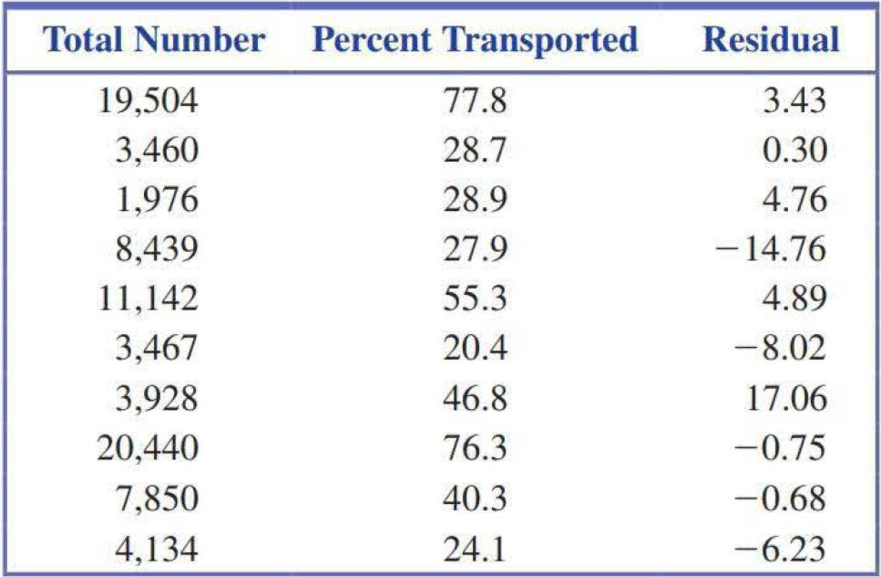
- a. The observation (3928, 46.8) has a large residual. Is this data point also an influential observation?
- b. The two points with unusually large x values (19,504 and 20,440) were not thought to be influential observations even though they are far removed in the x direction from the rest of the points in the
scatterplot . Explain why these two points are not influential. - c. Partial Minitab output resulting from fitting the least-squares line is shown here. What is the value of se? Write a sentence interpreting this value.
The regression equation is
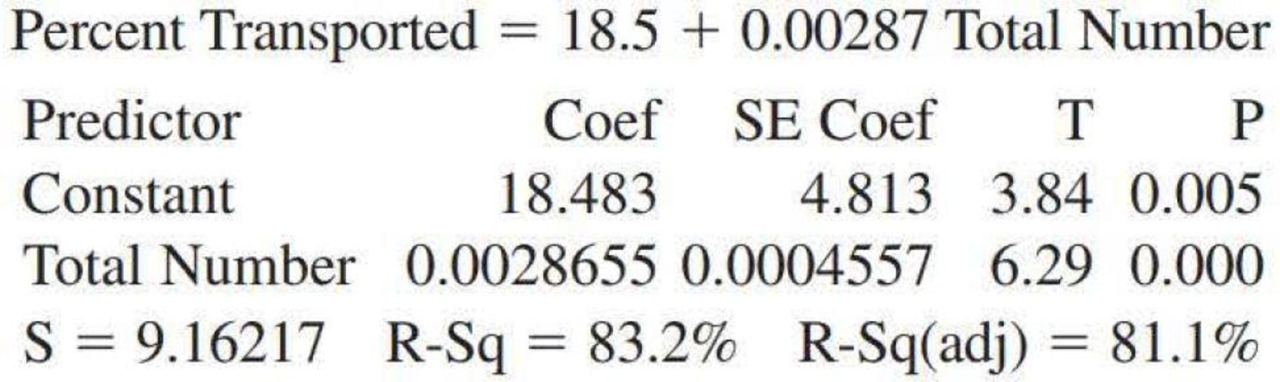
- d. What is the value of r2 for this data set (see Minitab output in Part (c))? Is the value of r2 large or small? Write a sentence interpreting the value of r2.
5.43 ● The relationship between x = Total number of salmon in a creek and y = Percentage of salmon killed by bears that were transported away from the stream prior to the bear eating the salmon was examined in the paper “Transportation of Pacific Salmon Carcasses from Streams to Riparian Forests by Bears” (Canadian Journal of Zoology [2009]: 195–203).
Data for the 10 years from 1999 to 2008 is given in the accompanying table.
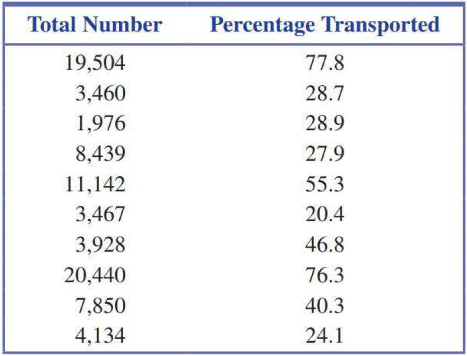
- a. Construct a scatterplot of the data.
- b. Does there appear to be a relationship between the total number of salmon in the stream and the percentage of salmon killed by bears that are transported away from the stream?
- c. Find the equation of the least-squares line. Draw the least-squares line on the scatterplot from Part (a).

Trending nowThis is a popular solution!

Chapter 5 Solutions
Introduction To Statistics And Data Analysis
Additional Math Textbook Solutions
Math in Our World
Elementary Statistics: Picturing the World (7th Edition)
Basic College Mathematics
Introductory Statistics
Precalculus: A Unit Circle Approach (3rd Edition)
APPLIED STAT.IN BUS.+ECONOMICS


- Name Harvard University California Institute of Technology Massachusetts Institute of Technology Stanford University Princeton University University of Cambridge University of Oxford University of California, Berkeley Imperial College London Yale University University of California, Los Angeles University of Chicago Johns Hopkins University Cornell University ETH Zurich University of Michigan University of Toronto Columbia University University of Pennsylvania Carnegie Mellon University University of Hong Kong University College London University of Washington Duke University Northwestern University University of Tokyo Georgia Institute of Technology Pohang University of Science and Technology University of California, Santa Barbara University of British Columbia University of North Carolina at Chapel Hill University of California, San Diego University of Illinois at Urbana-Champaign National University of Singapore…arrow_forwardA company found that the daily sales revenue of its flagship product follows a normal distribution with a mean of $4500 and a standard deviation of $450. The company defines a "high-sales day" that is, any day with sales exceeding $4800. please provide a step by step on how to get the answers in excel Q: What percentage of days can the company expect to have "high-sales days" or sales greater than $4800? Q: What is the sales revenue threshold for the bottom 10% of days? (please note that 10% refers to the probability/area under bell curve towards the lower tail of bell curve) Provide answers in the yellow cellsarrow_forwardFind the critical value for a left-tailed test using the F distribution with a 0.025, degrees of freedom in the numerator=12, and degrees of freedom in the denominator = 50. A portion of the table of critical values of the F-distribution is provided. Click the icon to view the partial table of critical values of the F-distribution. What is the critical value? (Round to two decimal places as needed.)arrow_forward
- A retail store manager claims that the average daily sales of the store are $1,500. You aim to test whether the actual average daily sales differ significantly from this claimed value. You can provide your answer by inserting a text box and the answer must include: Null hypothesis, Alternative hypothesis, Show answer (output table/summary table), and Conclusion based on the P value. Showing the calculation is a must. If calculation is missing,so please provide a step by step on the answers Numerical answers in the yellow cellsarrow_forwardShow all workarrow_forwardShow all workarrow_forward
 Linear Algebra: A Modern IntroductionAlgebraISBN:9781285463247Author:David PoolePublisher:Cengage Learning
 Functions and Change: A Modeling Approach to Coll...AlgebraISBN:9781337111348Author:Bruce Crauder, Benny Evans, Alan NoellPublisher:Cengage Learning
 Glencoe Algebra 1, Student Edition, 9780079039897...AlgebraISBN:9780079039897Author:CarterPublisher:McGraw Hill
 Holt Mcdougal Larson Pre-algebra: Student Edition...AlgebraISBN:9780547587776Author:HOLT MCDOUGALPublisher:HOLT MCDOUGAL
 Big Ideas Math A Bridge To Success Algebra 1: Stu...AlgebraISBN:9781680331141Author:HOUGHTON MIFFLIN HARCOURTPublisher:Houghton Mifflin Harcourt