Concept explainers
Videos
a.
Draw the plots of the proportion of bird eggs hatching for the lowlands and mid-elevation areas versus exposure time.
Identify whether the shapes of the plots are as expected in case of “logistic” plots.
a.
Answer to Problem 71E
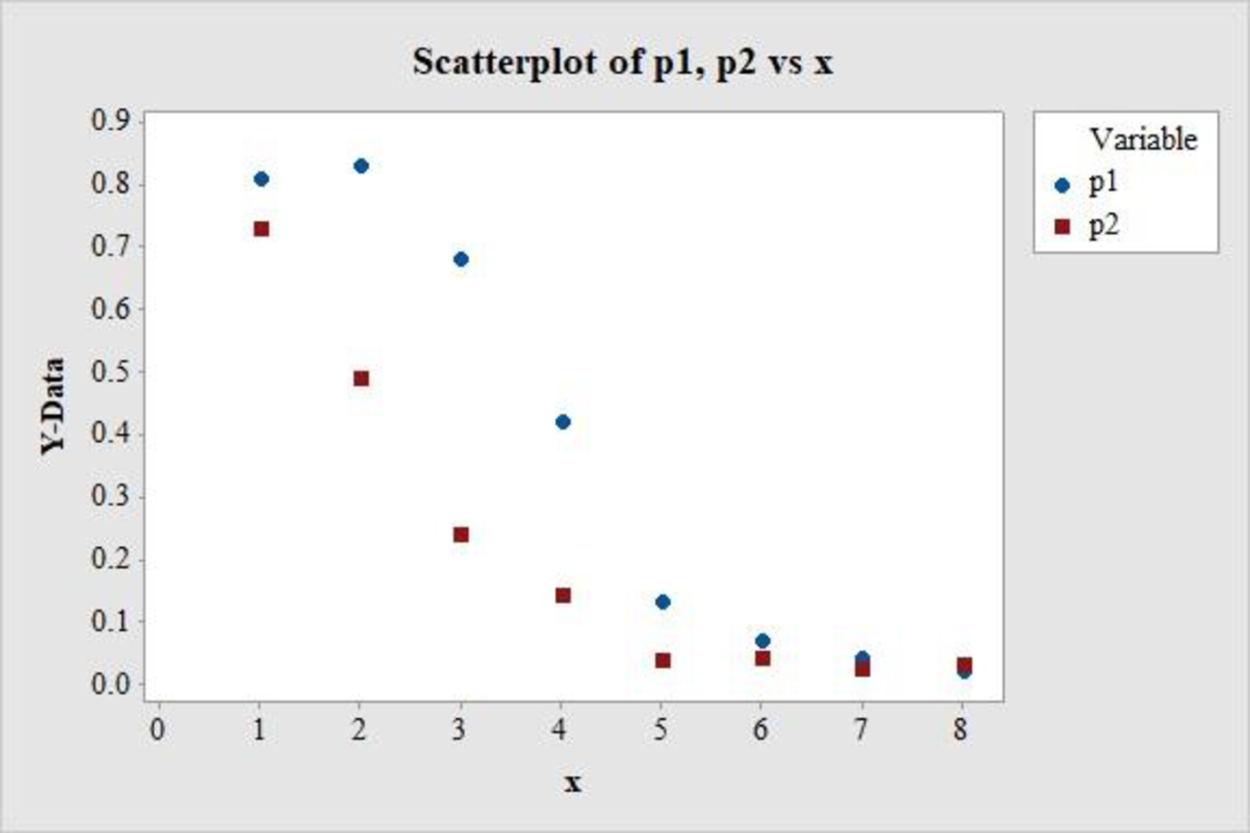
The plot of the proportion of bird eggs hatching for the lowlands and mid-elevation areas versus exposure time is as follows:
Explanation of Solution
Calculation:
The given data relates the proportion of bird eggs hatching for the lowlands, mid-elevation areas and cloud-forests with exposure time (days).
Denote the proportion of hatching for lowlands as
Software procedure:
Step-by-step procedure to draw the scatterplots using MINITAB software is given below:
- Choose Graph > Scatterplot.
- Choose Simple, and then click OK.
- Enter the column of p1 in the first cell under Y variables.
- Enter the column of x in the first cell under X variables.
- Enter the column of p2 in the second cell under Y variables.
- Enter the column of x in the second cell under X variables.
- Choose Multiple Graphs.
- Select Overlaid on the same graph under Show pairs of graph variables.
- Click OK in all dialogue boxes.
Thus, the scatterplot for the data is obtained.
The logistic plots usually have an approximate S-shaped distribution. In the above scatterplot, it is observed that both the proportions have approximately extended S-shaped distributions.
Hence, the shapes of the plots are more-or-less as expected in case of “logistic” plots.
b.
Find the value of
Fit a regression line of the form
Describe the significance of the negative slope.
b.
Answer to Problem 71E
The regression line fitted to the given data is
Explanation of Solution
Calculation:
Logistic regression:
The logistic regression equation for the prediction of a probability for the given value of the explanatory variable, x, is
The values of
Data transformation
Software procedure:
Step-by-step procedure to transform the data using MINITAB software is given below:
- Choose Calc > Calculator.
- Enter the column of y* under Store result in variable.
- Enter the formula LN(‘p3’/(1–‘p3’)) under Expression.
- Click OK.
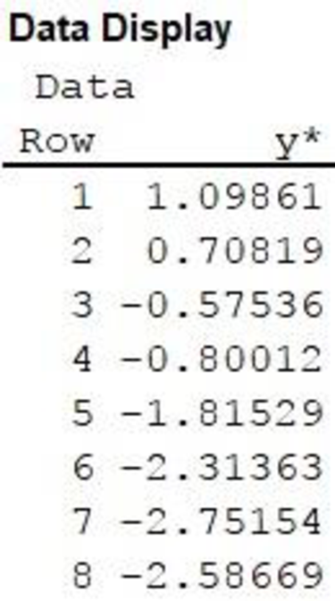
The transformed variable is stored in the column y*.
Data display:
Software procedure:
Step by step procedure to display the data using MINITAB software is given as,
- Choose Data > Display Data.
- Under Column, constants, and matrices to display, enter the column of y*.
- Click OK on all dialogue boxes.
The output using MINITAB software is given as follows:
Regression equation:
Software procedure:
Step by step procedure to obtain the regression equation using the MINITAB software:
- Choose Stat > Regression > Regression > Fit Regression Model.
- Enter the column of y* under Responses.
- Enter the columns of x under Continuous predictors.
- Choose Results and select Analysis of Variance, Model Summary, Coefficients, Regression Equation.
- Click OK in all dialogue boxes.
Output obtained using MINITAB is given below:
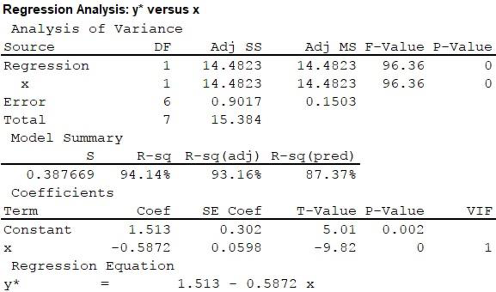
In the output, substituting
It is observed that the slope of x is –0.5872, which is negative. A negative slope implies that an increase in x causes a decrease in yꞌ.
Now, it is known that the quantity
In this case, an increase in exposure time decreases the natural logarithm of odds of hatching in the cloud forest area, which, in turn, implies a decrease in the odds of hatching.
Thus, the negative slope implies that an increase in exposure time causes a decrease in the odds of hatching of an egg in the cloud forest area.
c.
Predict the proportion of hatching in the cloud forest conditions, for an exposure time of 3 days.
Predict the proportion of hatching in the cloud forest conditions, for an exposure time of 5 days.
c.
Answer to Problem 71E
The proportion of hatching in the cloud forest conditions, for an exposure time of 3 days is 0.4382.
The proportion of hatching in the cloud forest conditions, for an exposure time of 5 days is 0.1942.
Explanation of Solution
Calculation:
For an exposure time of 3 days, substitute
Thus,
Thus, the proportion of hatching in the cloud forest conditions, for an exposure time of 3 days is 0.4382.
For an exposure time of 5 days, substitute
Thus,
Thus, the proportion of hatching in the cloud forest conditions, for an exposure time of 5 days is 0.1942.
d.
Identify the point of exposure time, at which, the proportion of hatching in the cloud forest conditions changes from greater than 0.5 to less than 0.5.
d.
Answer to Problem 71E
The exposure time, at which, the proportion of hatching in the cloud forest conditions changes from greater than 0.5 to less than 0.5 is 2.5766 days.
Explanation of Solution
Calculation:
For the proportion of hatching of 0.5, substitute
Thus,
As a result, the exposure time for the proportion of hatching of 0.5 is 2.5766 days.
Now, from the explanation in Part b, an increase in the exposure time causes a decrease in the odds of hatching in the cloud forest conditions. Thus, an increase in exposure time from 2.5766 days would cause a decrease in the proportion of hatching, whereas a decrease in exposure time from 2.5766 days would cause an increase in the proportion of hatching.
Thus, the exposure time, at which, the proportion of hatching in the cloud forest conditions changes from greater than 0.5 to less than 0.5 is 2.5766 days.
Want to see more full solutions like this?
Chapter 5 Solutions
Introduction to Statistics and Data Analysis


- Show that L′(θ) = Cθ394(1 −2θ)604(395 −2000θ).arrow_forwarda) Let X and Y be independent random variables both with the same mean µ=0. Define a new random variable W = aX +bY, where a and b are constants. (i) Obtain an expression for E(W).arrow_forwardThe table below shows the estimated effects for a logistic regression model with squamous cell esophageal cancer (Y = 1, yes; Y = 0, no) as the response. Smoking status (S) equals 1 for at least one pack per day and 0 otherwise, alcohol consumption (A) equals the average number of alcohoic drinks consumed per day, and race (R) equals 1 for blacks and 0 for whites. Variable Effect (β) P-value Intercept -7.00 <0.01 Alcohol use 0.10 0.03 Smoking 1.20 <0.01 Race 0.30 0.02 Race × smoking 0.20 0.04 Write-out the prediction equation (i.e., the logistic regression model) when R = 0 and again when R = 1. Find the fitted Y S conditional odds ratio in each case. Next, write-out the logistic regression model when S = 0 and again when S = 1. Find the fitted Y R conditional odds ratio in each case.arrow_forward
- The chi-squared goodness-of-fit test can be used to test if data comes from a specific continuous distribution by binning the data to make it categorical. Using the OpenIntro Statistics county_complete dataset, test the hypothesis that the persons_per_household 2019 values come from a normal distribution with mean and standard deviation equal to that variable's mean and standard deviation. Use signficance level a = 0.01. In your solution you should 1. Formulate the hypotheses 2. Fill in this table Range (-⁰⁰, 2.34] (2.34, 2.81] (2.81, 3.27] (3.27,00) Observed 802 Expected 854.2 The first row has been filled in. That should give you a hint for how to calculate the expected frequencies. Remember that the expected frequencies are calculated under the assumption that the null hypothesis is true. FYI, the bounderies for each range were obtained using JASP's drag-and-drop cut function with 8 levels. Then some of the groups were merged. 3. Check any conditions required by the chi-squared…arrow_forwardSuppose that you want to estimate the mean monthly gross income of all households in your local community. You decide to estimate this population parameter by calling 150 randomly selected residents and asking each individual to report the household’s monthly income. Assume that you use the local phone directory as the frame in selecting the households to be included in your sample. What are some possible sources of error that might arise in your effort to estimate the population mean?arrow_forwardFor the distribution shown, match the letter to the measure of central tendency. A B C C Drag each of the letters into the appropriate measure of central tendency. Mean C Median A Mode Barrow_forward
- A physician who has a group of 38 female patients aged 18 to 24 on a special diet wishes to estimate the effect of the diet on total serum cholesterol. For this group, their average serum cholesterol is 188.4 (measured in mg/100mL). Suppose that the total serum cholesterol measurements are normally distributed with standard deviation of 40.7. (a) Find a 95% confidence interval of the mean serum cholesterol of patients on the special diet.arrow_forwardThe accompanying data represent the weights (in grams) of a simple random sample of 10 M&M plain candies. Determine the shape of the distribution of weights of M&Ms by drawing a frequency histogram. Find the mean and median. Which measure of central tendency better describes the weight of a plain M&M? Click the icon to view the candy weight data. Draw a frequency histogram. Choose the correct graph below. ○ A. ○ C. Frequency Weight of Plain M and Ms 0.78 0.84 Frequency OONAG 0.78 B. 0.9 0.96 Weight (grams) Weight of Plain M and Ms 0.84 0.9 0.96 Weight (grams) ○ D. Candy Weights 0.85 0.79 0.85 0.89 0.94 0.86 0.91 0.86 0.87 0.87 - Frequency ☑ Frequency 67200 0.78 → Weight of Plain M and Ms 0.9 0.96 0.84 Weight (grams) Weight of Plain M and Ms 0.78 0.84 Weight (grams) 0.9 0.96 →arrow_forwardThe acidity or alkalinity of a solution is measured using pH. A pH less than 7 is acidic; a pH greater than 7 is alkaline. The accompanying data represent the pH in samples of bottled water and tap water. Complete parts (a) and (b). Click the icon to view the data table. (a) Determine the mean, median, and mode pH for each type of water. Comment on the differences between the two water types. Select the correct choice below and fill in any answer boxes in your choice. A. For tap water, the mean pH is (Round to three decimal places as needed.) B. The mean does not exist. Data table Тар 7.64 7.45 7.45 7.10 7.46 7.50 7.68 7.69 7.56 7.46 7.52 7.46 5.15 5.09 5.31 5.20 4.78 5.23 Bottled 5.52 5.31 5.13 5.31 5.21 5.24 - ☑arrow_forward
- く Chapter 5-Section 1 Homework X MindTap - Cengage Learning x + C webassign.net/web/Student/Assignment-Responses/submit?pos=3&dep=36701632&tags=autosave #question3874894_3 M Gmail 品 YouTube Maps 5. [-/20 Points] DETAILS MY NOTES BBUNDERSTAT12 5.1.020. ☆ B Verify it's you Finish update: All Bookmarks PRACTICE ANOTHER A computer repair shop has two work centers. The first center examines the computer to see what is wrong, and the second center repairs the computer. Let x₁ and x2 be random variables representing the lengths of time in minutes to examine a computer (✗₁) and to repair a computer (x2). Assume x and x, are independent random variables. Long-term history has shown the following times. 01 Examine computer, x₁₁ = 29.6 minutes; σ₁ = 8.1 minutes Repair computer, X2: μ₂ = 92.5 minutes; σ2 = 14.5 minutes (a) Let W = x₁ + x2 be a random variable representing the total time to examine and repair the computer. Compute the mean, variance, and standard deviation of W. (Round your answers…arrow_forwardThe acidity or alkalinity of a solution is measured using pH. A pH less than 7 is acidic; a pH greater than 7 is alkaline. The accompanying data represent the pH in samples of bottled water and tap water. Complete parts (a) and (b). Click the icon to view the data table. (a) Determine the mean, median, and mode pH for each type of water. Comment on the differences between the two water types. Select the correct choice below and fill in any answer boxes in your choice. A. For tap water, the mean pH is (Round to three decimal places as needed.) B. The mean does not exist. Data table Тар Bottled 7.64 7.45 7.46 7.50 7.68 7.45 7.10 7.56 7.46 7.52 5.15 5.09 5.31 5.20 4.78 5.52 5.31 5.13 5.31 5.21 7.69 7.46 5.23 5.24 Print Done - ☑arrow_forwardThe median for the given set of six ordered data values is 29.5. 9 12 23 41 49 What is the missing value? The missing value is ☐.arrow_forward
 Algebra & Trigonometry with Analytic GeometryAlgebraISBN:9781133382119Author:SwokowskiPublisher:Cengage
 Functions and Change: A Modeling Approach to Coll...AlgebraISBN:9781337111348Author:Bruce Crauder, Benny Evans, Alan NoellPublisher:Cengage Learning
 Glencoe Algebra 1, Student Edition, 9780079039897...AlgebraISBN:9780079039897Author:CarterPublisher:McGraw Hill