Videos
a.
Draw a
a.
Answer to Problem 18CRE
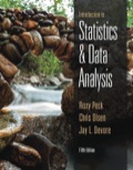
The scatterplot for the data is obtained as follows:
The relationship between the variables is nonlinear.
Explanation of Solution
Calculation:
The data on success (%), y and energy of shock, x is given.
Scatterplot:
Software procedure:
Step-by-step procedure to draw the scatterplot using MINITAB software is given below:
- Choose Graph > Scatterplot.
- Choose Simple, and then click OK.
- Enter the column of y under Y variables.
- Enter the column of x under X variables.
- Click OK.
Thus, the scatterplot is obtained.
A careful observation of the scatterplot reveals that for lower values of x, the points are close to being linear. However, the curvature in the distribution of the points gradually increases with increasing values of x.
Thus, the relationship between the variables is nonlinear.
b.
Fit a least-squares regression line to the data.
Construct a residual plot for the model.
Explain whether the residual plot supports the conclusion in Part a.
b.
Answer to Problem 18CRE
The least-squares regression line for the data is
Explanation of Solution
Calculation:
The least-squares regression line can be obtained using software.
Regression:
Software procedure:
Step by step procedure to get regression equation using MINITAB software is given as,
- Choose Stat > Regression > Regression > Fit Regression Model.
- Under Responses, enter the column of y.
- Under Continuous predictors, enter the columns of x.
- Choose Results and select Analysis of Variance, Model Summary, Coefficients, Regression Equation.
- Choose Graphs, under Residual versus the variables, enter x.
- Click OK on all dialogue boxes.
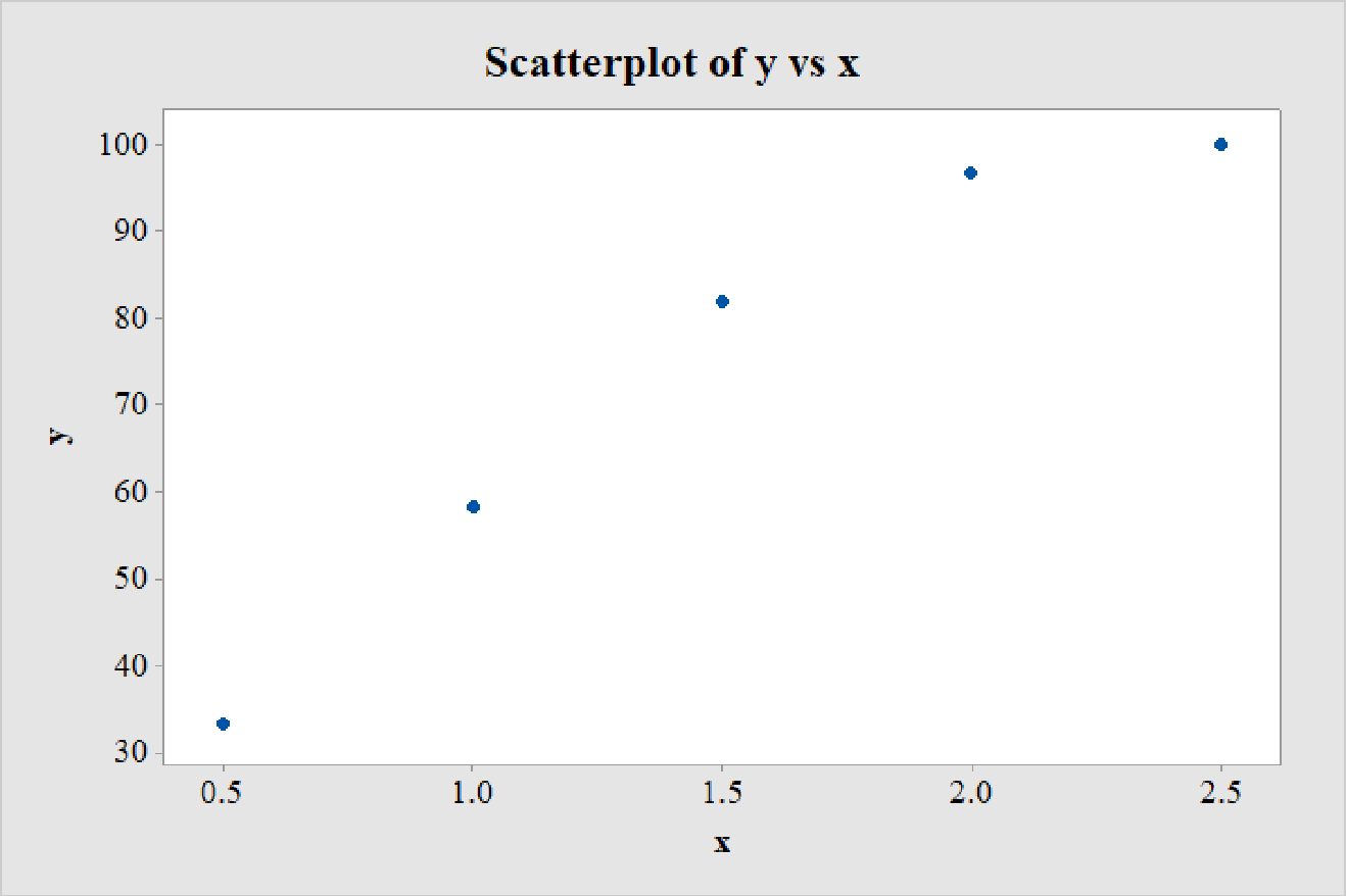
The outputs using MINITAB software is given as follows:
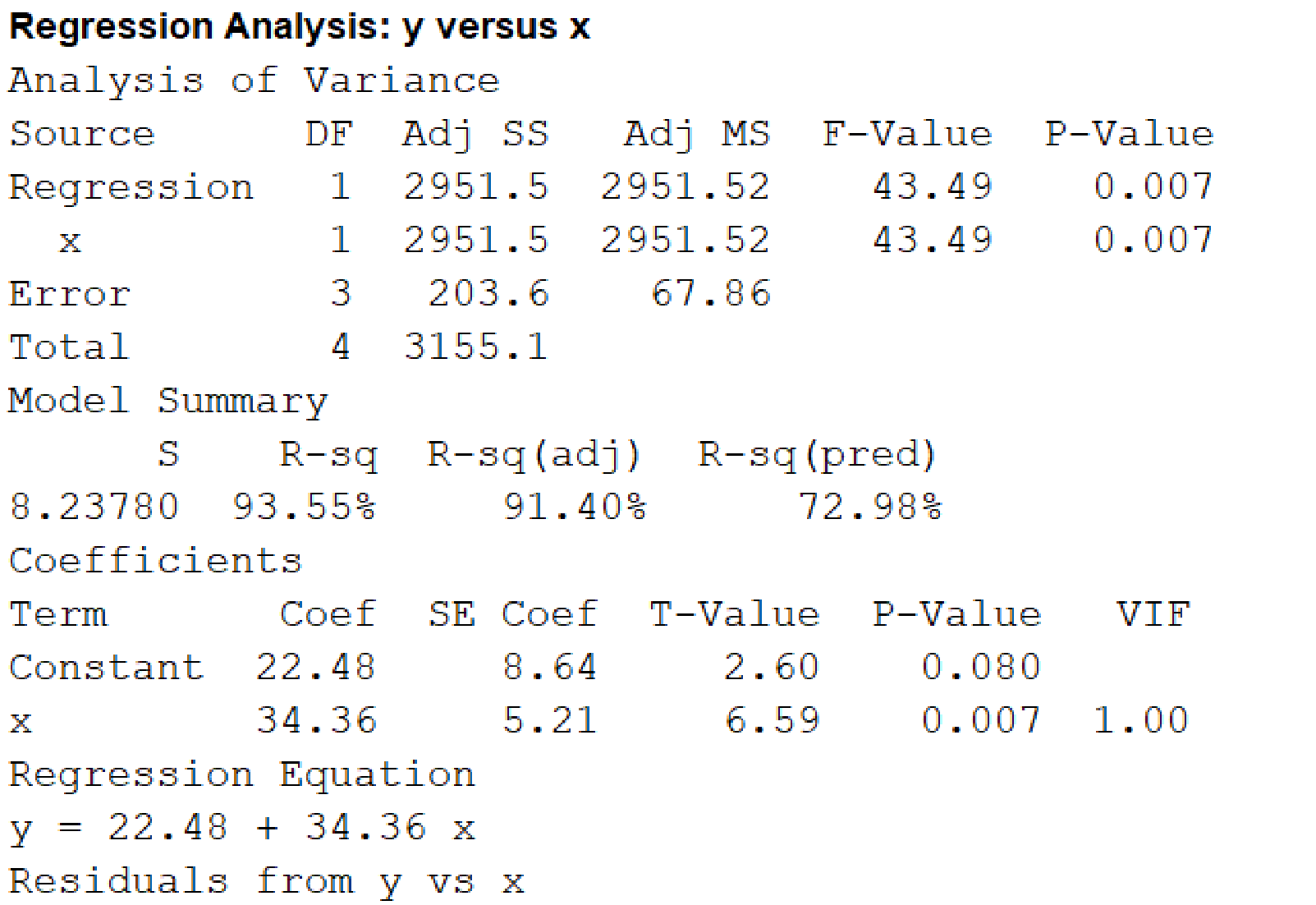
Residual plot:
From the output, the least-squares regression line is:
The ideal residual plot for a linear regression model must not show any pattern and must be randomly distributed. However, this residual plot clearly shows a curved pattern, with an approximate inverted U-shape. This suggests that the data is not linearly distributed.
Thus, the residual plot supports the conclusion in Part a.
c.
Justify whether the transformation
c.
Answer to Problem 18CRE
The transformation
Explanation of Solution
Calculation:
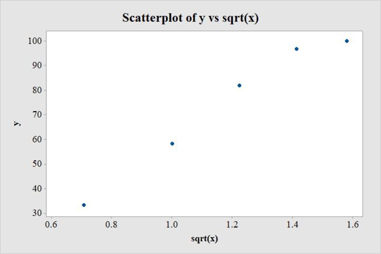
The suitable transformation can be identified by constructing scatterplot between y and
Consider the transformed variable,
Data transformation
Software procedure:
Step-by-step procedure to transform the data using MINITAB software is given below:
- Choose Calc > Calculator.
- Enter the column of sqrt(x) under Store result in variable.
- Enter the formula SQRT(‘x’) under Expression.
- Click OK.
The transformed variable is stored in the column sqrt(x).
Scatterplot:
Software procedure:
Step-by-step procedure to draw the scatterplot using MINITAB software is given below:
- Choose Graph > Scatterplot.
- Choose Simple, and then click OK.
- Enter the column of y under Y variables.
- Enter the column of sqrt(x) under X variables.
- Click OK.
The output obtained using MINITAB is as follows:
Consider the transformed variable,
Data transformation
Software procedure:
Step-by-step procedure to transform the data using MINITAB software is given below:
- Choose Calc > Calculator.
- Enter the column of sqrt(x) under Store result in variable.
- Enter the formula LOGTEN(‘x’) under Expression.
- Click OK.
The transformed variable is stored in the column log(x).
Scatterplot:
Software procedure:
Step-by-step procedure to draw the scatterplot using MINITAB software is given below:
- Choose Graph > Scatterplot.
- Choose Simple, and then click OK.
- Enter the column of y under Y variables.
- Enter the column of log(x) under X variables.
- Click OK.
The output obtained using MINITAB is as follows:
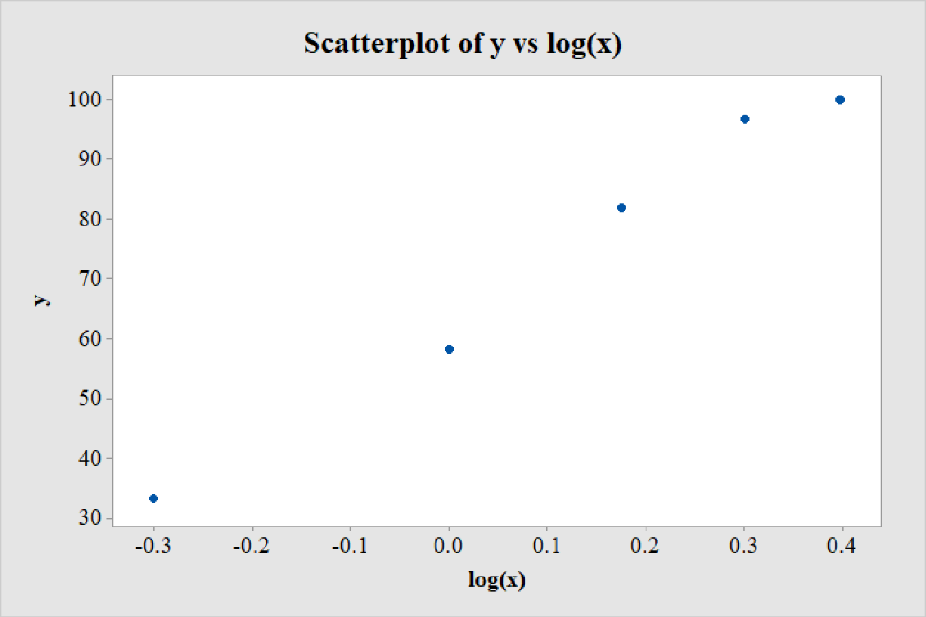
A careful observation of the scatterplot between y and
On the other hand, the scatterplot between y and
Thus, the transformation
d.
Find the least-squares regression line between y and the transformation recommended in the previous part.
d.
Answer to Problem 18CRE
The least-squares regression equation between y and the transformation recommended in the previous part, that is,
Explanation of Solution
Calculation:
The least-squares regression line can be obtained using software.
Regression:
Software procedure:
Step by step procedure to get regression equation using MINITAB software is given as,
- Choose Stat > Regression > Regression > Fit Regression Model.
- Under Responses, enter the column of y.
- Under Continuous predictors, enter the columns of log(x).
- Choose Results and select Analysis of Variance, Model Summary, Coefficients, Regression Equation.
- Click OK on all dialogue boxes.
The outputs using MINITAB software is given as follows:
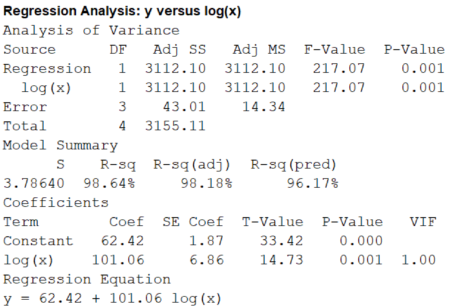
From the output, the least-squares regression equation between y and the transformation recommended in the previous part, that is,
e.
Predict the success for an energy shock 1.75 times the threshold.
Predict the success for an energy shock 0.8 times the threshold.
e.
Answer to Problem 18CRE
The success for an energy shock 1.75 times the threshold is 86.98%.
The success for an energy shock 0.8 times the threshold is 52.63%.
Explanation of Solution
Calculation:
The energy of shock is given as a multiple of the threshold of defibrillation.
For an energy shock 1.75 times the threshold,
Thus, the success for an energy shock 1.75 times the threshold is 86.98%.
For an energy shock 0.8 times the threshold,
Thus, the success for an energy shock 0.8 times the threshold is 52.63%.
Want to see more full solutions like this?
Chapter 5 Solutions
Introduction to Statistics and Data Analysis


- Hi, I need to sort out where I went wrong. So, please us the data attached and run four separate regressions, each using the Recruiters rating as the dependent variable and GMAT, Accept Rate, Salary, and Enrollment, respectively, as a single independent variable. Interpret this equation. Round your answers to four decimal places, if necessary. If your answer is negative number, enter "minus" sign. Equation for GMAT: Ŷ = _______ + _______ GMAT Equation for Accept Rate: Ŷ = _______ + _______ Accept Rate Equation for Salary: Ŷ = _______ + _______ Salary Equation for Enrollment: Ŷ = _______ + _______ Enrollmentarrow_forwardQuestion 21 of 28 (1 point) | Question Attempt: 5 of Unlimited Dorothy ✔ ✓ 12 ✓ 13 ✓ 14 ✓ 15 ✓ 16 ✓ 17 ✓ 18 ✓ 19 ✓ 20 = 21 22 > How many apps? According to a website, the mean number of apps on a smartphone in the United States is 82. Assume the number of apps is normally distributed with mean 82 and standard deviation 30. Part 1 of 2 (a) What proportion of phones have more than 47 apps? Round the answer to four decimal places. The proportion of phones that have more than 47 apps is 0.8783 Part: 1/2 Try again kip Part ی E Recheck == == @ W D 80 F3 151 E R C レ Q FA 975 % T B F5 10 の 000 园 Save For Later Submit Assignment © 2025 McGraw Hill LLC. All Rights Reserved. Terms of Use | Privacy Center | Accessibility Y V& U H J N * 8 M I K O V F10 P = F11 F12 . darrow_forwardYou are provided with data that includes all 50 states of the United States. Your task is to draw a sample of: 20 States using Random Sampling (2 points: 1 for random number generation; 1 for random sample) 10 States using Systematic Sampling (4 points: 1 for random numbers generation; 1 for generating random sample different from the previous answer; 1 for correct K value calculation table; 1 for correct sample drawn by using systematic sampling) (For systematic sampling, do not use the original data directly. Instead, first randomize the data, and then use the randomized dataset to draw your sample. Furthermore, do not use the random list previously generated, instead, generate a new random sample for this part. For more details, please see the snapshot provided at the end.) You are provided with data that includes all 50 states of the United States. Your task is to draw a sample of: o 20 States using Random Sampling (2 points: 1 for random number generation; 1 for random sample) o…arrow_forward
- Course Home ✓ Do Homework - Practice Ques ✓ My Uploads | bartleby + mylab.pearson.com/Student/PlayerHomework.aspx?homeworkId=688589738&questionId=5&flushed=false&cid=8110079¢erwin=yes Online SP 2025 STA 2023-009 Yin = Homework: Practice Questions Exam 3 Question list * Question 3 * Question 4 ○ Question 5 K Concluir atualização: Ava Pearl 04/02/25 9:28 AM HW Score: 71.11%, 12.09 of 17 points ○ Points: 0 of 1 Save Listed in the accompanying table are weights (kg) of randomly selected U.S. Army male personnel measured in 1988 (from "ANSUR I 1988") and different weights (kg) of randomly selected U.S. Army male personnel measured in 2012 (from "ANSUR II 2012"). Assume that the two samples are independent simple random samples selected from normally distributed populations. Do not assume that the population standard deviations are equal. Complete parts (a) and (b). Click the icon to view the ANSUR data. a. Use a 0.05 significance level to test the claim that the mean weight of the 1988…arrow_forwardsolving problem 1arrow_forwardselect bmw stock. you can assume the price of the stockarrow_forward
- This problem is based on the fundamental option pricing formula for the continuous-time model developed in class, namely the value at time 0 of an option with maturity T and payoff F is given by: We consider the two options below: Fo= -rT = e Eq[F]. 1 A. An option with which you must buy a share of stock at expiration T = 1 for strike price K = So. B. An option with which you must buy a share of stock at expiration T = 1 for strike price K given by T K = T St dt. (Note that both options can have negative payoffs.) We use the continuous-time Black- Scholes model to price these options. Assume that the interest rate on the money market is r. (a) Using the fundamental option pricing formula, find the price of option A. (Hint: use the martingale properties developed in the lectures for the stock price process in order to calculate the expectations.) (b) Using the fundamental option pricing formula, find the price of option B. (c) Assuming the interest rate is very small (r ~0), use Taylor…arrow_forwardDiscuss and explain in the picturearrow_forwardBob and Teresa each collect their own samples to test the same hypothesis. Bob’s p-value turns out to be 0.05, and Teresa’s turns out to be 0.01. Why don’t Bob and Teresa get the same p-values? Who has stronger evidence against the null hypothesis: Bob or Teresa?arrow_forward
- Review a classmate's Main Post. 1. State if you agree or disagree with the choices made for additional analysis that can be done beyond the frequency table. 2. Choose a measure of central tendency (mean, median, mode) that you would like to compute with the data beyond the frequency table. Complete either a or b below. a. Explain how that analysis can help you understand the data better. b. If you are currently unable to do that analysis, what do you think you could do to make it possible? If you do not think you can do anything, explain why it is not possible.arrow_forward0|0|0|0 - Consider the time series X₁ and Y₁ = (I – B)² (I – B³)Xt. What transformations were performed on Xt to obtain Yt? seasonal difference of order 2 simple difference of order 5 seasonal difference of order 1 seasonal difference of order 5 simple difference of order 2arrow_forwardCalculate the 90% confidence interval for the population mean difference using the data in the attached image. I need to see where I went wrong.arrow_forward
 Glencoe Algebra 1, Student Edition, 9780079039897...AlgebraISBN:9780079039897Author:CarterPublisher:McGraw Hill