Chapter 4.5, Problem 101E

a.

To determine

To graph the sine function and its polynomial approximation in the same viewing window and compares the graphs using the graphing utility.

Answer to Problem 101E

The polynomial function is a good approximation of the sine function for x- values near 0

Explanation of Solution

Given information: The sine and cosine functions can be approximated by the

Polynomials,$\sin x\approx x-\frac{x^3}{3!}+\frac{x^5}{5!}and\cos x\approx 1-\frac{x^2}{2!}+\frac{x^4}{4!}$

where x is in radian.

Calculation:

The graph of sine function and its polynomial approximation is given below.

  

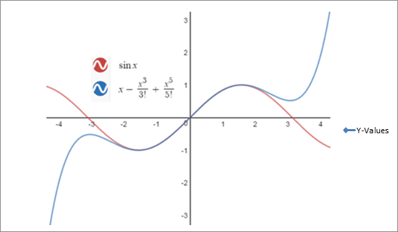
The polynomial function is a good approximation of the sine function for x- values near 0.

b.

To determine

To graph the cosine function and its polynomial approximation in the same viewing window and compares the graphs using the graphing utility.

Answer to Problem 101E

The polynomial function is a good approximation of the cosine function for x- values near 0.

Explanation of Solution

Given information: The sine and cosine functions can be approximated by the

Polynomials,$\sin x\approx x-\frac{x^3}{3!}+\frac{x^5}{5!}and\cos x\approx 1-\frac{x^2}{2!}+\frac{x^4}{4!}$

where x is in radian.

Calculation:

c.

To determine

To study the patterns in the polynomial approximations of the sine and cosine functions and predict the next term each. Then repeat parts (a) and (b) and find how did the accuracy of the approximations changes when an additional term was added.

Answer to Problem 101E

The accuracy increase in both case when the term is added.

Explanation of Solution

Given information: The sine and cosine functions can be approximated by the

Polynomials,$\sin x\approx x-\frac{x^3}{3!}+\frac{x^5}{5!}and\cos x\approx 1-\frac{x^2}{2!}+\frac{x^4}{4!}$

where x is in radian.

Calculation:

The sign is alternating & both the exponents & factorial increases by 2 for each term so:

  $\begin{array}{l}\sin x\approx x-\frac{x^3}{31}+\frac{x^5}{5!}-\frac{x^7}{7!}\\ \cos x\approx 1-\frac{x^2}{2!}+\frac{x^4}{4!}-\frac{x^6}{6!}\end{array}$

Using a graphing utility,

  

  

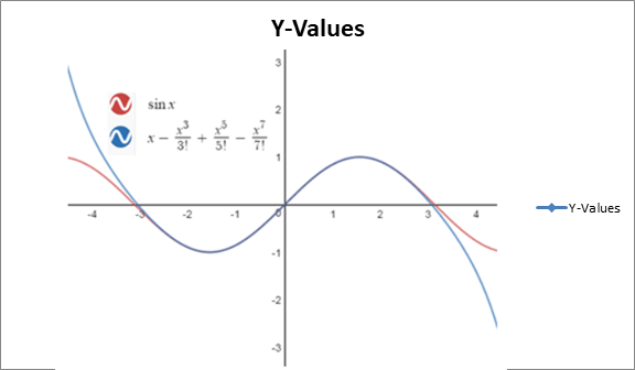
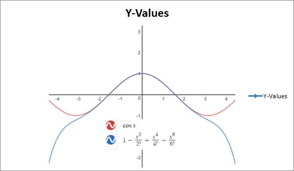
The accuracy increase in both case when the term is added.