
Concept explainers
Videos
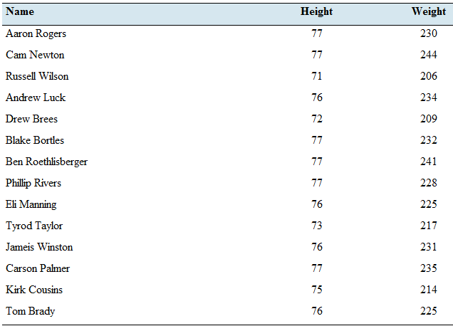
Pass the ball: The following table lists the heights (inches) and weights (pounds) of 14 National Football League quarterbacks in the 2016 season.
- Compute the least-squares regression line for predicting weight from height.
- Is it possible to interpret the y-intercept? Explain.
- If two quarterbacks differ in height by two inches: by how much would you predict their weights to differ?
- Predict the of a quarterback who is 74.5 inches tall.
- Kirk Cousins is 75 inches tall and weighs 214 pounds. Does he weigh more or less than the weight predicted by the least-squares regression line?
a.
To find: The least-square regression line for the given data set.
Answer to Problem 23E
The least square regression line of the given data set is,
Explanation of Solution
Following table with the heights and the weights of the national football quarterbacks in the season
| Name | Height | Weight |
| Aaron Rogers | 77 | 230 |
| Cam Newton | 77 | 244 |
| Russell Wilson | 71 | 206 |
| Andrew Luck | 76 | 234 |
| Drew Brees | 72 | 209 |
| Blake Bortles | 77 | 232 |
| Ben Roethlisberger | 77 | 241 |
| Philip Rivers | 77 | 228 |
| Eli Manning | 76 | 225 |
| Tyrod Taylor | 73 | 217 |
| Jamies Winston | 76 | 231 |
| Carson Palmer | 77 | 235 |
| Kirk Cousins | 75 | 214 |
| Tom Brady | 76 | 225 |
Calculation:
The least-square regression is given by the formula,
Where
The correlation coefficient is given by the formula,
Let
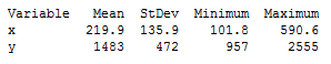
The correlation coefficient can be obtained by the following table.
Hence, the correlation coefficient is,
Then, the coefficient
Therefore,
Conclusion:
The least square regression line is found to be,
b.
To explain:The possibility to interpret the
Answer to Problem 23E
The
Explanation of Solution
The least-square regression line has been computed as
Considering the
The
Conclusion:
There is no chance to a weight be a negative value. Therefore, this
c.
To calculate:The difference in the weight of two players when their heights differ by two inches.
Answer to Problem 23E
The difference of weight is found to be
Explanation of Solution
The least-square regression line has been computed as
Calculation:
Let the height of the shorter payer be
Also, the weight of the taller player should be,
Simplifying the obtained weight,
Therefore, the difference of two weights should be,
Interpretation:
As the calculation above, the weight difference for two inches change in the height is found to be
d.
To find:The predicted weight of a player whose height is
Answer to Problem 23E
The weight of a player whose height is
Explanation of Solution
Calculation:
By the computed least-square regression line, we can calculate the predictions for the weights of the players by substituting their heights into the formula.
Here, the height is said to be
Conclusion:
The weight of a player whose height is
e.
To find:Whether theactual weight of this player is greater than the predicted weight or not.
Answer to Problem 23E
The player weighs less than the predicted weight.
Explanation of Solution
The player is
Calculation:
When the height is said to be
The predicted weight is found to be
Conclusion:
Since
Want to see more full solutions like this?
Chapter 4 Solutions
ELEMENTARY STATISTICS-ALEKS ACCESS CODE


- Faye cuts the sandwich in two fair shares to her. What is the first half s1arrow_forwardQuestion 2. An American option on a stock has payoff given by F = f(St) when it is exercised at time t. We know that the function f is convex. A person claims that because of convexity, it is optimal to exercise at expiration T. Do you agree with them?arrow_forwardQuestion 4. We consider a CRR model with So == 5 and up and down factors u = 1.03 and d = 0.96. We consider the interest rate r = 4% (over one period). Is this a suitable CRR model? (Explain your answer.)arrow_forward
- Question 3. We want to price a put option with strike price K and expiration T. Two financial advisors estimate the parameters with two different statistical methods: they obtain the same return rate μ, the same volatility σ, but the first advisor has interest r₁ and the second advisor has interest rate r2 (r1>r2). They both use a CRR model with the same number of periods to price the option. Which advisor will get the larger price? (Explain your answer.)arrow_forwardQuestion 5. We consider a put option with strike price K and expiration T. This option is priced using a 1-period CRR model. We consider r > 0, and σ > 0 very large. What is the approximate price of the option? In other words, what is the limit of the price of the option as σ∞. (Briefly justify your answer.)arrow_forwardQuestion 6. You collect daily data for the stock of a company Z over the past 4 months (i.e. 80 days) and calculate the log-returns (yk)/(-1. You want to build a CRR model for the evolution of the stock. The expected value and standard deviation of the log-returns are y = 0.06 and Sy 0.1. The money market interest rate is r = 0.04. Determine the risk-neutral probability of the model.arrow_forward
- Several markets (Japan, Switzerland) introduced negative interest rates on their money market. In this problem, we will consider an annual interest rate r < 0. We consider a stock modeled by an N-period CRR model where each period is 1 year (At = 1) and the up and down factors are u and d. (a) We consider an American put option with strike price K and expiration T. Prove that if <0, the optimal strategy is to wait until expiration T to exercise.arrow_forwardWe consider an N-period CRR model where each period is 1 year (At = 1), the up factor is u = 0.1, the down factor is d = e−0.3 and r = 0. We remind you that in the CRR model, the stock price at time tn is modeled (under P) by Sta = So exp (μtn + σ√AtZn), where (Zn) is a simple symmetric random walk. (a) Find the parameters μ and σ for the CRR model described above. (b) Find P Ste So 55/50 € > 1). StN (c) Find lim P 804-N (d) Determine q. (You can use e- 1 x.) Ste (e) Find Q So (f) Find lim Q 004-N StN Soarrow_forwardIn this problem, we consider a 3-period stock market model with evolution given in Fig. 1 below. Each period corresponds to one year. The interest rate is r = 0%. 16 22 28 12 16 12 8 4 2 time Figure 1: Stock evolution for Problem 1. (a) A colleague notices that in the model above, a movement up-down leads to the same value as a movement down-up. He concludes that the model is a CRR model. Is your colleague correct? (Explain your answer.) (b) We consider a European put with strike price K = 10 and expiration T = 3 years. Find the price of this option at time 0. Provide the replicating portfolio for the first period. (c) In addition to the call above, we also consider a European call with strike price K = 10 and expiration T = 3 years. Which one has the highest price? (It is not necessary to provide the price of the call.) (d) We now assume a yearly interest rate r = 25%. We consider a Bermudan put option with strike price K = 10. It works like a standard put, but you can exercise it…arrow_forward
- In this problem, we consider a 2-period stock market model with evolution given in Fig. 1 below. Each period corresponds to one year (At = 1). The yearly interest rate is r = 1/3 = 33%. This model is a CRR model. 25 15 9 10 6 4 time Figure 1: Stock evolution for Problem 1. (a) Find the values of up and down factors u and d, and the risk-neutral probability q. (b) We consider a European put with strike price K the price of this option at time 0. == 16 and expiration T = 2 years. Find (c) Provide the number of shares of stock that the replicating portfolio contains at each pos- sible position. (d) You find this option available on the market for $2. What do you do? (Short answer.) (e) We consider an American put with strike price K = 16 and expiration T = 2 years. Find the price of this option at time 0 and describe the optimal exercising strategy. (f) We consider an American call with strike price K ○ = 16 and expiration T = 2 years. Find the price of this option at time 0 and describe…arrow_forward2.2, 13.2-13.3) question: 5 point(s) possible ubmit test The accompanying table contains the data for the amounts (in oz) in cans of a certain soda. The cans are labeled to indicate that the contents are 20 oz of soda. Use the sign test and 0.05 significance level to test the claim that cans of this soda are filled so that the median amount is 20 oz. If the median is not 20 oz, are consumers being cheated? Click the icon to view the data. What are the null and alternative hypotheses? OA. Ho: Medi More Info H₁: Medi OC. Ho: Medi H₁: Medi Volume (in ounces) 20.3 20.1 20.4 Find the test stat 20.1 20.5 20.1 20.1 19.9 20.1 Test statistic = 20.2 20.3 20.3 20.1 20.4 20.5 Find the P-value 19.7 20.2 20.4 20.1 20.2 20.2 P-value= (R 19.9 20.1 20.5 20.4 20.1 20.4 Determine the p 20.1 20.3 20.4 20.2 20.3 20.4 Since the P-valu 19.9 20.2 19.9 Print Done 20 oz 20 oz 20 oz 20 oz ce that the consumers are being cheated.arrow_forwardT Teenage obesity (O), and weekly fast-food meals (F), among some selected Mississippi teenagers are: Name Obesity (lbs) # of Fast-foods per week Josh 185 10 Karl 172 8 Terry 168 9 Kamie Andy 204 154 12 6 (a) Compute the variance of Obesity, s²o, and the variance of fast-food meals, s², of this data. [Must show full work]. (b) Compute the Correlation Coefficient between O and F. [Must show full work]. (c) Find the Coefficient of Determination between O and F. [Must show full work]. (d) Obtain the Regression equation of this data. [Must show full work]. (e) Interpret your answers in (b), (c), and (d). (Full explanations required). Edit View Insert Format Tools Tablearrow_forward
 Glencoe Algebra 1, Student Edition, 9780079039897...AlgebraISBN:9780079039897Author:CarterPublisher:McGraw Hill
 Big Ideas Math A Bridge To Success Algebra 1: Stu...AlgebraISBN:9781680331141Author:HOUGHTON MIFFLIN HARCOURTPublisher:Houghton Mifflin Harcourt
 Holt Mcdougal Larson Pre-algebra: Student Edition...AlgebraISBN:9780547587776Author:HOLT MCDOUGALPublisher:HOLT MCDOUGAL
 Functions and Change: A Modeling Approach to Coll...AlgebraISBN:9781337111348Author:Bruce Crauder, Benny Evans, Alan NoellPublisher:Cengage Learning