Chapter 4, Problem 99CE

a.

To determine

Arrange the data and obtain X_min and X_max.

Answer to Problem 99CE

The value of X_min is 0.9.

The value of X_max is 11.9.

Explanation of Solution

Calculation:

The data state to choose a dataset to prepare a brief descriptive report.

Here, the data chosen is Data set A.

The Data set A represents the percentage of sales in selected industries.

The data set A of sales percent can be sorted either ascending or descending.

Here, the data is sorted in the ascending order.

Sorting:

Software procedure:

Step-by-step procedure to sort the data using the MINITAB software is given below:

• Choose Data > Sort.
• In columns to sort by, enter Percent.
• Under Columns to sort , Choose specified columns.
• In columns, enter the percent and choose increasing option.
• In storage location for current columns, choose “specified columns of the current worksheet”.
• In columns, enter “sorted percent”.
• Click ok.

Thus, the sorted data has been stored in the column of sorted percent.

Minimum and Maximum:

Step-by-step procedure to find the minimum and maximum using the MINITAB software using the given below:

• Choose Calc>calculator.
• In store result in variable box, enter Minimum.
• Under Expression, enter “MIN(Percent)”.
• Click ok.
• Choose Calc>calculator.
• In store result in variable box, enter Maximum.
• Under Expression, enter “MAX(Percent)”.
• Click ok.

Data display:

Step-by-step procedure to display the data using the MINITAB software using the given below:

• Choose data> display data.
• Select the columns to display as Minimum, Maximum.
• Click ok.

Output using the MINITAB software is given below:

• 

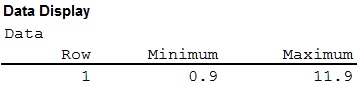
Thus, the value of X_min is 0.9 and the value of X_max is 11.9.

b.

To determine

Construct a histogram.

Answer to Problem 99CE

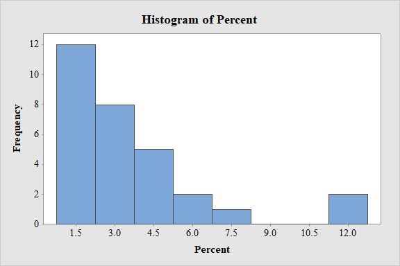
Histogram:

Output obtained from MINITAB software is:

Explanation of Solution

Calculation:

Software procedure:

• Step by step procedure to draw the Histogram using MINITAB software is given below:
• Choose Graph > Histogram.
• Choose Simple, and then click OK.
• In Graph variables, enter the Percent.
• Click OK.

Thus, the histogram has been obtained.

By observing the graph, it is clear that the curve is right skewed. Hence, it is appropriate to conclude that the data is approximately right skewed. Thus, the data set A for percent of sales is approximately right skewed.

c.

To determine

Find the mean and median.

Answer to Problem 99CE

The mean score is 3.55.

The median score is 3.

Explanation of Solution

Mean and median:

Software procedure:

Step-by-step procedure to find the mean, the median using the MINITAB software is given below:

• Choose Stat > Basic Statistics > Display Descriptive Statistics.
• In Variables enter the columns Percent.
• Choose option statistics, and select Mean, Median.
• Click OK.

Output using the MINITAB software is given below:

• 
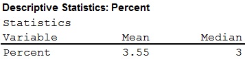
• Thus, the mean and the median for the data set A are 3.55 and 3 respectively.

Shape of the distribution:

• For symmetric data, the mean, the median and the mode are equal.
• For positively skewed data, the mean exceeds the median.
• For negatively skewed data, the mean is lower than the median.

From the value of mean, median, it is observed that the value of mean is greater than that of the median.

Thus, the data is said to be right skewed or positively skewed.

d.

To determine

Find the standard deviation for data set A.

Answer to Problem 99CE

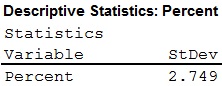
The standard deviation for data set A is 2.749.

Explanation of Solution

Standard deviation:

Software procedure:

Step-by-step procedure to find the mean and standard deviation using the MINITAB software is given below:

• Choose Stat > Basic Statistics > Display Descriptive Statistics.
• In Variables enter the columns Percent.
• Choose option statistics, and select Standard deviation.
• Click OK.

Output using the MINITAB software is given below:

• 
• Thus, the standard deviation have been obtained.

e.

To determine

Standardize the data and identify the outliers and unusual observations.

Answer to Problem 99CE

The standardized values of dataset A are given below:

-0.9640	-0.6366	0.3456	0.3820	-0.6730	0.0909
0.7093	-0.0182	-0.0182	-0.9276	-0.1637	-0.2001
1.4005	-0.9640	-0.8912	-0.0182	3.0375	-0.6002
-0.8185	1.0367	-0.2001	-0.4547	0.2728	-0.6366
-0.8912	-0.5638	-0.5638	0.4911	-0.3820	2.8192

There are one outlier in the dataset.

Explanation of Solution

Standardized values:

Software procedure:

Step-by-step software procedure to obtain standardized values using EXCEL software is as follows:

• Open an EXCEL file.
• Enter the data in the column A in cells A1 to A32.
• In cell B1, enter the formula “=STANDARDIZE(A1, 3.55, 2.749)”.
• Select “ENTER” option.
• Select and copy the cell B1 and drag till the 30^nd cell.
• Output using EXCEL software is given below:

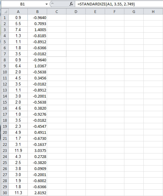
Thus, the standardized values have been obtained using EXCEL.

The outliers in the data set A can be identified using Empirical rule.

Empirical Rule:

The Empirical Rule for a Normal model states that:

• Within 1 standard deviation of mean, 68.26% of all observations will lie.
• Within 2 standard deviations of mean, 95.44% of all observations will lie.
• Within 3 standard deviations of mean, 99.73% of all observations will lie.

Empirical rule using MEGASTAT:

Software procedure:

Step-by-step software procedure to obtain Empirical rule using Mega Stat software is as follows:

• Open an EXCEL file.
• Enter the data in the column A in cells A1 to A30.
• From the Add-Ins, Select Mega Stat >Descriptive statistics.
• A dialogue box appears.
• In Input range box, select the input range from Sheet1!$A$1:$A$30.
• From the list box, select Empirical rule.
• Click “OK”.

Output obtained using MEGA STAT is as follows:

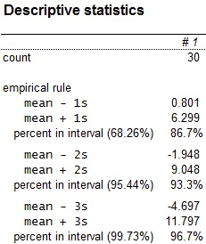
The upper and lower bounds for the intervals indicated by the Empirical rule have been obtained.

Based on the z-scores, the observation has one outlier, that is, the observations with values 11.9 do not lie within the 3-standard deviations limits (–4.697 to 11.797). there is no unusual observation in the data set A.

f.

To determine

Find the quartiles and a box plot for data set A.

Answer to Problem 99CE

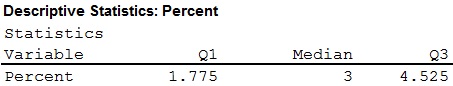
The Q₁ (25^th percentile) is 1.775, Q₂ (50^th percentile) is 3 and Q₃ (75^th percentile) is 4.525.

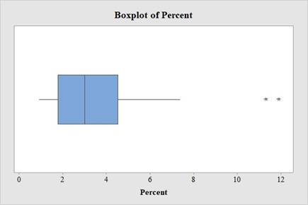
The boxplot for the data set A is:

Explanation of Solution

Quartiles:

Software procedure:

Step-by-step procedure to find the Quartiles using the MINITAB software:

• Choose Stat > Basic Statistics > Display Descriptive Statistics.
• In Variables enter the columns Percent.
• Choose option statistics, and select First Quartile, Median and Third Quartile.
• Choose option Graphs, and select boxplot of data.
• Click OK.

Output using the MINITAB software is given below:

• 
• 
• Thus, the Quartiles and boxplot have been obtained.

Observation:

From the boxplot, it is observed that the data set has two outliers within it. The boxplot disclosed that the median is closer to the first quartile, Q₁ than it is to the third quartile, Q₃, suggesting that the data is right skewed. The whiskers on the two sides are close in length, although it appears that the left whisker is slightly longer.