Videos
Laplace Transforms
In the last few chapters, we have looked at several ways to use
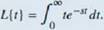
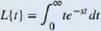
The Laplace transform is defined in terms of an integral as
7
e""
ft
Note that the input to a Laplace transform is a function of time, /(/), and the output is a function of frequency, F(j), Although many real-world examples require the use of
Let's stan with a simple example. Here we calculate the Laplace transform of /(f) = t. We have
This is an improper integral, so we express it in terms of a limit, which gives
Now we use integration by pans to evaluate the integral. Note that we are integrating with respect to t, so we treat the variable s as a constant. We have
u—t dv — dt
du=dt v
— — ye_ir.
Then we obtain
= + +
= ~K + °1 -
= JinL[[-i,-]-±[e--lj]
- c + c
= 0-0 + -L
s“
_x
2* s
1. Calculate the Laplace transform of /(/) = 1.
3.Calculate the Laplace transform of /(/) = : (Note, you will have to integrate by parts twice.)
Laplace transforms are often used to solve differential equations. Differential equations are not covered in detail until later in this book; but, for now, let’s look at the relationship between the Laplace transform of a function and the Laplace transform of its derivative.
Let’s start with the definition of the Laplace transform. We have
WW! = r™ r'
= lim / e~st fifth.
4.Use integration by parts to evaluate Jjm^ e~sl fifth. (Let « = /{/) and dv — e '!dt.) After integrating by parts and evaluating the limit, you should see that
Then,
Thus, differentiation in the time domain simplifies to multiplication by s in the frequency domain.
The final thing we look at in this project is how the Laplace transforms of fit] and its antiderivative are
related. Let g(r) — f(u}dii. Then,
¦'o
lim /
;-* caj" 5.Use integration by parts to evaluate hrn^y e ’ g(t)dl. (Let u = gif) and dv = e dt. Note, by the way,
that we have defined gif, du — fifth.)
As you might expect, you should see that
L|^(r)| = |-L[/(/)i.
Integration in the time domain simplifies to division by s in ±e frequency domain.
Want to see the full answer?
Check out a sample textbook solution
Chapter 3 Solutions
Calculus Volume 2
Additional Math Textbook Solutions
A First Course in Probability (10th Edition)
Calculus: Early Transcendentals (2nd Edition)
A Problem Solving Approach To Mathematics For Elementary School Teachers (13th Edition)
Elementary Statistics: Picturing the World (7th Edition)
University Calculus: Early Transcendentals (4th Edition)


- Suppose that a particle moves along a straight line with velocity v (t) = 62t, where 0 < t <3 (v(t) in meters per second, t in seconds). Find the displacement d (t) at time t and the displacement up to t = 3. d(t) ds = ["v (s) da = { The displacement up to t = 3 is d(3)- meters.arrow_forwardLet f (x) = x², a 3, and b = = 4. Answer exactly. a. Find the average value fave of f between a and b. fave b. Find a point c where f (c) = fave. Enter only one of the possible values for c. c=arrow_forwardThe following data represent total ventilation measured in liters of air per minute per square meter of body area for two independent (and randomly chosen) samples. Analyze these data using the appropriate non-parametric hypothesis testarrow_forward
- each column represents before & after measurements on the same individual. Analyze with the appropriate non-parametric hypothesis test for a paired design.arrow_forwardShould you be confident in applying your regression equation to estimate the heart rate of a python at 35°C? Why or why not?arrow_forwardGiven your fitted regression line, what would be the residual for snake #5 (10 C)?arrow_forward
- Calculate the 95% confidence interval around your estimate of r using Fisher’s z-transformation. In your final answer, make sure to back-transform to the original units.arrow_forwardCalculate Pearson’s correlation coefficient (r) between temperature and heart rate.arrow_forwardCalculate the least squares regression line and write the equation.arrow_forward
 Algebra & Trigonometry with Analytic GeometryAlgebraISBN:9781133382119Author:SwokowskiPublisher:Cengage