Shown, again, in the following table is world population, in billions, for seven selected years from 1950 through 2010. Using a graphing utility's logistic regression option, we obtain the equation shown on the screen. We see from the calculator screen at the bottom of the previous page that a logistic growth model for world population, f(x), in billions, x years after 1949 is f ( x ) = 12.57 1 + 4.11 e − 0.026 x Use this function to solve Exercises 38-42. When did world population reach 7 billion?
Shown, again, in the following table is world population, in billions, for seven selected years from 1950 through 2010. Using a graphing utility's logistic regression option, we obtain the equation shown on the screen. We see from the calculator screen at the bottom of the previous page that a logistic growth model for world population, f(x), in billions, x years after 1949 is f ( x ) = 12.57 1 + 4.11 e − 0.026 x Use this function to solve Exercises 38-42. When did world population reach 7 billion?
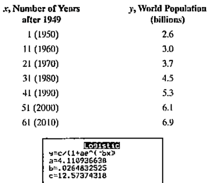
Shown, again, in the following table is world population, in billions, for seven selected years from 1950 through 2010. Using a graphing utility's logistic regression option, we obtain the equation shown on the screen.
We see from the calculator screen at the bottom of the previous page that a logistic growth model for world population, f(x), in billions, x years after 1949 is
Show that the Laplace equation in Cartesian coordinates:
J²u
J²u
+
= 0
მx2 Jy2
can be reduced to the following form in cylindrical polar coordinates:
湯(
ди
1 8²u
+
Or 7,2 მ)2
= 0.
Find integrating factor
Draw the vertical and horizontal asymptotes. Then plot the intercepts (if any), and plot at least one point on each side of each vertical asymptote.
Need a deep-dive on the concept behind this application? Look no further. Learn more about this topic, calculus and related others by exploring similar questions and additional content below.
01 - What Is A Differential Equation in Calculus? Learn to Solve Ordinary Differential Equations.; Author: Math and Science;https://www.youtube.com/watch?v=K80YEHQpx9g;License: Standard YouTube License, CC-BY
Higher Order Differential Equation with constant coefficient (GATE) (Part 1) l GATE 2018; Author: GATE Lectures by Dishank;https://www.youtube.com/watch?v=ODxP7BbqAjA;License: Standard YouTube License, CC-BY


 Algebra & Trigonometry with Analytic GeometryAlgebraISBN:9781133382119Author:SwokowskiPublisher:Cengage
 Glencoe Algebra 1, Student Edition, 9780079039897...AlgebraISBN:9780079039897Author:CarterPublisher:McGraw Hill
 College Algebra (MindTap Course List)AlgebraISBN:9781305652231Author:R. David Gustafson, Jeff HughesPublisher:Cengage Learning
 Linear Algebra: A Modern IntroductionAlgebraISBN:9781285463247Author:David PoolePublisher:Cengage Learning