Videos
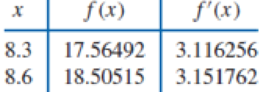
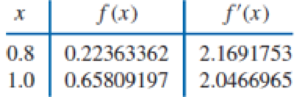
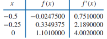
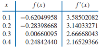
Use Theorem 3.9 or Algorithm 3.3 to construct an approximating polynomial for the following data.
ALGORITHM 3.3
Hermite Interpolation
To obtain the coefficients of the Hermite interpolating polynomial H(x) on the (n + 1) distinct numbers x0, …, xn for the function f:
INPUT numbers x0, x1, …, xn; values f (x0), ... , f (xn) and f′ (x0), ... , f′ (xn).
OUTPUT the numbers Q0, 0, Q1, 1, … , Q2n + 1, 2n + 1 where
Step 1 For i = 0, 1, … , n do Steps 2 and 3.
Step 2
Step 3 If i ≠ 0 then set
Step 4 For i = 2, 3, … , 2n + 1
for j = 2, 3, ... , i set
Step 5 OUTPUT (Q0, 0, Q1, 1, … , Q2n + 1, 2n + 1);
STOP.
Theorem 3.9 If f ∈ C1 [a, b] and x0, …, xn ∈ [a, b] are distinct, the unique polynomial of least degree agreeing with f and f′ at x0, …, xn is the Hermite polynomial of degree at most 2n + 1 given by
where, for Ln, j (x) denoting the jth Lagrange coefficient polynomial of degree n, we have
Moreover, if f ∈ C2n + 2 [a, b], then
for some (generally unknown) ξ(x) in the interval (a, b).
Want to see the full answer?
Check out a sample textbook solution
Chapter 3 Solutions
Numerical Analysis


- For each of the time series, construct a line chart of the data and identify the characteristics of the time series (that is, random, stationary, trend, seasonal, or cyclical). Month Number (Thousands)Dec 1991 65.60Jan 1992 71.60Feb 1992 78.80Mar 1992 111.60Apr 1992 107.60May 1992 115.20Jun 1992 117.80Jul 1992 106.20Aug 1992 109.90Sep 1992 106.00Oct 1992 111.80Nov 1992 84.50Dec 1992 78.60Jan 1993 70.50Feb 1993 74.60Mar 1993 95.50Apr 1993 117.80May 1993 120.90Jun 1993 128.50Jul 1993 115.30Aug 1993 121.80Sep 1993 118.50Oct 1993 123.30Nov 1993 102.30Dec 1993 98.70Jan 1994 76.20Feb 1994 83.50Mar 1994 134.30Apr 1994 137.60May 1994 148.80Jun 1994 136.40Jul 1994 127.80Aug 1994 139.80Sep 1994 130.10Oct 1994 130.60Nov 1994 113.40Dec 1994 98.50Jan 1995 84.50Feb 1995 81.60Mar 1995 103.80Apr 1995 116.90May 1995 130.50Jun 1995 123.40Jul 1995 129.10Aug 1995…arrow_forwardFor each of the time series, construct a line chart of the data and identify the characteristics of the time series (that is, random, stationary, trend, seasonal, or cyclical). Year Month Units1 Nov 42,1611 Dec 44,1862 Jan 42,2272 Feb 45,4222 Mar 54,0752 Apr 50,9262 May 53,5722 Jun 54,9202 Jul 54,4492 Aug 56,0792 Sep 52,1772 Oct 50,0872 Nov 48,5132 Dec 49,2783 Jan 48,1343 Feb 54,8873 Mar 61,0643 Apr 53,3503 May 59,4673 Jun 59,3703 Jul 55,0883 Aug 59,3493 Sep 54,4723 Oct 53,164arrow_forwardConsider the table of values below. x y 2 64 3 48 4 36 5 27 Fill in the right side of the equation y= with an expression that makes each ordered pari (x,y) in the table a solution to the equation.arrow_forward
- Consider the following system of equations, Ax=b : x+2y+3z - w = 2 2x4z2w = 3 -x+6y+17z7w = 0 -9x-2y+13z7w = -14 a. Find the solution to the system. Write it as a parametric equation. You can use a computer to do the row reduction. b. What is a geometric description of the solution? Explain how you know. c. Write the solution in vector form? d. What is the solution to the homogeneous system, Ax=0?arrow_forward2. Find a matrix A with the following qualities a. A is 3 x 3. b. The matrix A is not lower triangular and is not upper triangular. c. At least one value in each row is not a 1, 2,-1, -2, or 0 d. A is invertible.arrow_forwardFind the exact area inside r=2sin(2\theta ) and outside r=\sqrt(3)arrow_forward
 Algebra & Trigonometry with Analytic GeometryAlgebraISBN:9781133382119Author:SwokowskiPublisher:Cengage
 Mathematics For Machine TechnologyAdvanced MathISBN:9781337798310Author:Peterson, John.Publisher:Cengage Learning,
 Linear Algebra: A Modern IntroductionAlgebraISBN:9781285463247Author:David PoolePublisher:Cengage Learning
 Elements Of Modern AlgebraAlgebraISBN:9781285463230Author:Gilbert, Linda, JimmiePublisher:Cengage Learning,