
Videos
Size of Dams These data represent the volumes in cubic yards of the largest dams in the United States and in South America. Construct a boxplot of the data for each region and compare the distributions.
| United States | South America |
| 125,628 92,000 78,008 77,700 66,500 62,850 52,435 50,000 |
311,539 274,026 105,944 102,014 56,242 46,563 |
The boxplot of the given data and comparison of the distribution.
Answer to Problem 16E
The boxplot for the capacity of dams in the United States is shown below,
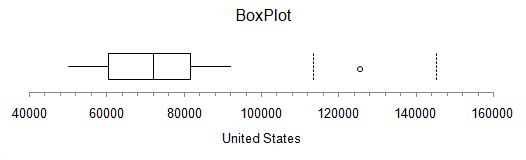
Fig (1)
The boxplot for the capacity of dams in the South America is shown below,
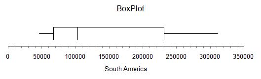
Fig (2)
The range and variation of the capacity of the dams in South America is larger than the capacity of the dams in United Stated.
Explanation of Solution
Given info:
The data of the capacity of dams in the United States and the South America is shown in the table below.
| United States | South America |
| 125628 | 311539 |
| 92000 | 274026 |
| 78008 | 105944 |
| 77700 | 102014 |
| 66500 | 56242 |
| 62850 | 46563 |
| 52435 | |
| 50000 |
Calculation:
The boxplot is used to graphically depict groups of numerical data through their quantities.
Arrange the densities of dams in the United States in ascending order as shown below.
| United States |
| 50000 |
| 52435 |
| 62850 |
| 66500 |
| 77700 |
| 78008 |
| 92000 |
| 125628 |
The minimum capacity of the dam from the above table is 50000 and the maximum capacity of the dam is 125628.
The number of data in the table is 8.
The formula to calculate the median for even data is shown below.
The total number of terms in the data is 8 so, substitute 8 for n in the above formula.
Substitute 66500 for
Thus, the median of the data is 72,100.
Software procedure:
Step-by-step procedure to construct boxplot by using Excel add-in (MegaStat).
- First select the data for which boxplot is obtained.
- Click on Add-Ins option in the top.
- Click on MegaStat option on the left side of the screen and then click on descriptive statistics.
- Select the boxplot option then in input range, select the data cells and then click ok.
Observation:
Since median falls to the right of the centre of the box thus the distribution is slightly negatively skewed.
Now, arrange the data of densities of dams in the South America in ascending order as shown below.
| South America |
| 46563 |
| 56242 |
| 102014 |
| 105944 |
| 274026 |
| 311539 |
The minimum capacity of the dam from the above table is 46563 and the maximum capacity of the dam is 311539.
The number of data in the table is 6.
The formula to calculate the median for even data is shown below.
The total number of terms in the data is 6 so, substitute 6 for n in the above formula.
Substitute 102014 for
Thus, the median of the data is 103,979.
Software procedure:
Step-by-step procedure to construct boxplot by using Excel add-in (MegaStat).
- First select the data for which boxplot is obtained.
- Click on Add-Ins option in the top.
- Click on MegaStat option on the left side of the screen and then click on descriptive statistics.
- Select the boxplot option then in input range, select the data cells and then click ok.
Observation:
Since median falls to the left of the centre of the box thus the distribution is slightly positively skewed.
The range and variation of the capacity of the dams in South America is larger than the capacity of the dams in United Stated.
Want to see more full solutions like this?
Chapter 3 Solutions
ELEMENTARY STATISTICS W/CONNECT >IP<


- Suppose a random sample of 459 married couples found that 307 had two or more personality preferences in common. In another random sample of 471 married couples, it was found that only 31 had no preferences in common. Let p1 be the population proportion of all married couples who have two or more personality preferences in common. Let p2 be the population proportion of all married couples who have no personality preferences in common. Find a95% confidence interval for . Round your answer to three decimal places.arrow_forwardA history teacher interviewed a random sample of 80 students about their preferences in learning activities outside of school and whether they are considering watching a historical movie at the cinema. 69 answered that they would like to go to the cinema. Let p represent the proportion of students who want to watch a historical movie. Determine the maximal margin of error. Use α = 0.05. Round your answer to three decimal places. arrow_forwardA random sample of medical files is used to estimate the proportion p of all people who have blood type B. If you have no preliminary estimate for p, how many medical files should you include in a random sample in order to be 99% sure that the point estimate will be within a distance of 0.07 from p? Round your answer to the next higher whole number.arrow_forward
- A clinical study is designed to assess the average length of hospital stay of patients who underwent surgery. A preliminary study of a random sample of 70 surgery patients’ records showed that the standard deviation of the lengths of stay of all surgery patients is 7.5 days. How large should a sample to estimate the desired mean to within 1 day at 95% confidence? Round your answer to the whole number.arrow_forwardA clinical study is designed to assess the average length of hospital stay of patients who underwent surgery. A preliminary study of a random sample of 70 surgery patients’ records showed that the standard deviation of the lengths of stay of all surgery patients is 7.5 days. How large should a sample to estimate the desired mean to within 1 day at 95% confidence? Round your answer to the whole number.arrow_forwardIn the experiment a sample of subjects is drawn of people who have an elbow surgery. Each of the people included in the sample was interviewed about their health status and measurements were taken before and after surgery. Are the measurements before and after the operation independent or dependent samples?arrow_forward
- iid 1. The CLT provides an approximate sampling distribution for the arithmetic average Ỹ of a random sample Y₁, . . ., Yn f(y). The parameters of the approximate sampling distribution depend on the mean and variance of the underlying random variables (i.e., the population mean and variance). The approximation can be written to emphasize this, using the expec- tation and variance of one of the random variables in the sample instead of the parameters μ, 02: YNEY, · (1 (EY,, varyi n For the following population distributions f, write the approximate distribution of the sample mean. (a) Exponential with rate ẞ: f(y) = ß exp{−ßy} 1 (b) Chi-square with degrees of freedom: f(y) = ( 4 ) 2 y = exp { — ½/ } г( (c) Poisson with rate λ: P(Y = y) = exp(-\} > y! y²arrow_forward2. Let Y₁,……., Y be a random sample with common mean μ and common variance σ². Use the CLT to write an expression approximating the CDF P(Ỹ ≤ x) in terms of µ, σ² and n, and the standard normal CDF Fz(·).arrow_forwardmatharrow_forward
- Compute the median of the following data. 32, 41, 36, 42, 29, 30, 40, 22, 25, 37arrow_forwardTask Description: Read the following case study and answer the questions that follow. Ella is a 9-year-old third-grade student in an inclusive classroom. She has been diagnosed with Emotional and Behavioural Disorder (EBD). She has been struggling academically and socially due to challenges related to self-regulation, impulsivity, and emotional outbursts. Ella's behaviour includes frequent tantrums, defiance toward authority figures, and difficulty forming positive relationships with peers. Despite her challenges, Ella shows an interest in art and creative activities and demonstrates strong verbal skills when calm. Describe 2 strategies that could be implemented that could help Ella regulate her emotions in class (4 marks) Explain 2 strategies that could improve Ella’s social skills (4 marks) Identify 2 accommodations that could be implemented to support Ella academic progress and provide a rationale for your recommendation.(6 marks) Provide a detailed explanation of 2 ways…arrow_forwardQuestion 2: When John started his first job, his first end-of-year salary was $82,500. In the following years, he received salary raises as shown in the following table. Fill the Table: Fill the following table showing his end-of-year salary for each year. I have already provided the end-of-year salaries for the first three years. Calculate the end-of-year salaries for the remaining years using Excel. (If you Excel answer for the top 3 cells is not the same as the one in the following table, your formula / approach is incorrect) (2 points) Geometric Mean of Salary Raises: Calculate the geometric mean of the salary raises using the percentage figures provided in the second column named “% Raise”. (The geometric mean for this calculation should be nearly identical to the arithmetic mean. If your answer deviates significantly from the mean, it's likely incorrect. 2 points) Starting salary % Raise Raise Salary after raise 75000 10% 7500 82500 82500 4% 3300…arrow_forward
 Glencoe Algebra 1, Student Edition, 9780079039897...AlgebraISBN:9780079039897Author:CarterPublisher:McGraw Hill
 Holt Mcdougal Larson Pre-algebra: Student Edition...AlgebraISBN:9780547587776Author:HOLT MCDOUGALPublisher:HOLT MCDOUGAL
 Big Ideas Math A Bridge To Success Algebra 1: Stu...AlgebraISBN:9781680331141Author:HOUGHTON MIFFLIN HARCOURTPublisher:Houghton Mifflin Harcourt
 Algebra: Structure And Method, Book 1AlgebraISBN:9780395977224Author:Richard G. Brown, Mary P. Dolciani, Robert H. Sorgenfrey, William L. ColePublisher:McDougal Littell