
a.
To construct: A percentile graph for the given data.
a.
Answer to Problem 3.3.23RE
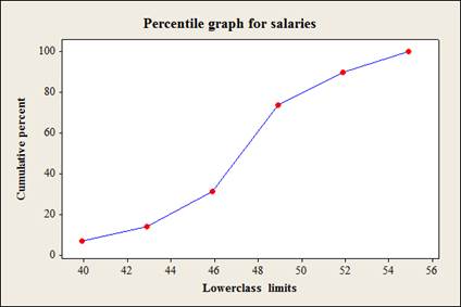
The percentile graph for the given data is as follows,
Explanation of Solution
Given info:
The data represents the salaries (in millions of dollars) for 29 NFL teams for the 1999 2000 season.
| Class limits | Frequency |
| 39.9-42.8 | 2 |
| 42.9-45.8 | 2 |
| 45.9-48.8 | 5 |
| 48.9-51.8 | 5 |
| 51.8-54.8 | 12 |
| 54.9-57.8 | 3 |
Calculation:
The cumulative frequency for the distribution is calculated and tabulated below,
| Class limits | Frequency | Cumulative frequency |
| 39.9-42.8 | 2 | 2 |
| 42.9-45.8 | 2 |
|
| 45.9-48.8 | 5 |
|
| 48.9-51.8 | 5 |
|
| 51.8-54.8 | 12 |
|
| 54.9-57.8 | 3 |
|
The formula to calculate the cumulative percentage is as follows,
For the cumulative frequency 2:
Substitute cumulative frequency as 2 and n as 29 in the formula,
Similarly for remaining values the cumulative percent are tabulated below
| Class limit | Frequency |
Cumulative frequency | Cumulative percent |
| 39.9-42.8 | 2 | 2 | 6.89 |
| 42.9-45.8 | 2 | 4 |
|
| 45.9-48.8 | 5 | 9 |
|
| 48.9-51.8 | 5 | 14 |
|
| 51.9-54.8 | 12 | 26 |
|
| 54.9-57.8 | 3 | 29 |
|
|
|
Software procedure:
Step-by-step software procedure to draw ogive curve using MINITAB software is as follows:
- Choose Graph >
Scatter plot . - Choose With Connect Line, and then click OK.
- In Y variables, enter the Cumulative Percent.
- In X variables enter the Lower class limits.
- In Data view, select Symbols and Connect line under Data display.
- In Data view, select Smoother and enter 0 for Degree of smoothing and 1 for Number of steps under Lowness.
- Click OK
- To modify the interval settings, double click on the horizontal axis of the graph. Then, select Labels > Specified. In this box, enter the values for the cutpoints of the bin intervals (39.9, 42.9, 45.9, 48.9, 51.9, 54.9).
b.
The values that correspond to the 35th, 65th and 85th percentiles.
b.
Answer to Problem 3.3.23RE
The values corresponding to 35th, 65th and 85th percentile are 50, 53 and 55.
Explanation of Solution
Calculation:
From part (a) the cumulative percent table is as follows,
| Class limit | Frequency |
Cumulative frequency |
Cumulative percent |
| 39.9-42.8 | 2 | 2 | 6.89 |
| 42.9-45.8 | 2 | 4 | 13.79 |
| 45.9-48.8 | 5 | 9 | 31.03 |
| 48.9-51.8 | 5 | 14 | 73.68 |
| 51.9-54.8 | 12 | 26 | 89.65 |
| 54.9-57.8 | 3 | 29 | 100 |
|
|
For 35th percentile:
The 35th percentile location is calculated below,
Substitute n as 29 and m as 35 in the formula,
Here the 10th observation corresponds to the cumulative frequency 14 which falls in the class 48.9-51.8.
The formula to calculate the percentile for the grouped data is given below,
Where,
- l, the lower limit of the class.
- h, the width of class.
- f, the frequency of the class.
- p, the percentiles rank.
- n is the total number
- c is the preceding cumulative frequency
Substitute 35 for m, 48.9 for
Thus, the 35th percentile of the data is approximately 50.
For 65th percentile:
The 65th percentile location is calculated below,
Substitute n as 29 and m as 65 in the formula,
Here the 19th observation corresponds to the cumulative frequency 26 which falls in the class 51.9-54.8.
Substitute 65 for m, 51.9 for
Thus, the 65th percentile of the data is approximately 53.
For 85th percentile:
The 85th percentile location is calculated below,
Substitute n as 29 and m as 85 in the formula,
Here the 25th observation corresponds to the cumulative frequency 26 which falls in the class 51.9-54.8.
Substitute 85 for m, 51.9 for
Thus, the 85th percentile of the data is approximately 55.
c.
The percentile rank of values 44, 48 and 54.
c.
Answer to Problem 3.3.23RE
The percentile rank for values 44, 48 and 54 are 10th, 26th and 78th respectively.
Explanation of Solution
Calculation:
| Class limit | Frequency |
Cumulative frequency |
| 39.9-42.8 | 2 | 2 |
| 42.9-45.8 | 2 | 4 |
| 45.9-48.8 | 5 | 9 |
| 48.9-51.8 | 5 | 14 |
| 51.9-54.8 | 12 | 26 |
| 54.9-57.8 | 3 | 29 |
|
|
For the value 44:
Here, the value 44 falls in the interval 42.9-45.8.
Substitute 44 for
Thus, the percentile rank for the value 44 is 10th percentile.
For the value 48:
Here, the value 48 falls in the interval 45.9-48.8
Substitute 48 for
Thus, the percentile rank for the value 48 is 26th percentile.
For the value 48:
Here, the value 48 falls in the interval 51.9-54.8
Substitute 54 for
Thus, the percentile rank for the value 54 is 78th percentile
Want to see more full solutions like this?
Chapter 3 Solutions
ELEMENTARY STATISTICS W/CONNECT >IP<

- 21. ANALYSIS OF LAST DIGITS Heights of statistics students were obtained by the author as part of an experiment conducted for class. The last digits of those heights are listed below. Construct a frequency distribution with 10 classes. Based on the distribution, do the heights appear to be reported or actually measured? Does there appear to be a gap in the frequencies and, if so, how might that gap be explained? What do you know about the accuracy of the results? 3 4 555 0 0 0 0 0 0 0 0 0 1 1 23 3 5 5 5 5 5 5 5 5 5 5 5 5 6 6 8 8 8 9arrow_forwardA side view of a recycling bin lid is diagramed below where two panels come together at a right angle. 45 in 24 in Width? — Given this information, how wide is the recycling bin in inches?arrow_forward1 No. 2 3 4 Binomial Prob. X n P Answer 5 6 4 7 8 9 10 12345678 8 3 4 2 2552 10 0.7 0.233 0.3 0.132 7 0.6 0.290 20 0.02 0.053 150 1000 0.15 0.035 8 7 10 0.7 0.383 11 9 3 5 0.3 0.132 12 10 4 7 0.6 0.290 13 Poisson Probability 14 X lambda Answer 18 4 19 20 21 22 23 9 15 16 17 3 1234567829 3 2 0.180 2 1.5 0.251 12 10 0.095 5 3 0.101 7 4 0.060 3 2 0.180 2 1.5 0.251 24 10 12 10 0.095arrow_forward
- step by step on Microssoft on how to put this in excel and the answers please Find binomial probability if: x = 8, n = 10, p = 0.7 x= 3, n=5, p = 0.3 x = 4, n=7, p = 0.6 Quality Control: A factory produces light bulbs with a 2% defect rate. If a random sample of 20 bulbs is tested, what is the probability that exactly 2 bulbs are defective? (hint: p=2% or 0.02; x =2, n=20; use the same logic for the following problems) Marketing Campaign: A marketing company sends out 1,000 promotional emails. The probability of any email being opened is 0.15. What is the probability that exactly 150 emails will be opened? (hint: total emails or n=1000, x =150) Customer Satisfaction: A survey shows that 70% of customers are satisfied with a new product. Out of 10 randomly selected customers, what is the probability that at least 8 are satisfied? (hint: One of the keyword in this question is “at least 8”, it is not “exactly 8”, the correct formula for this should be = 1- (binom.dist(7, 10, 0.7,…arrow_forwardKate, Luke, Mary and Nancy are sharing a cake. The cake had previously been divided into four slices (s1, s2, s3 and s4). What is an example of fair division of the cake S1 S2 S3 S4 Kate $4.00 $6.00 $6.00 $4.00 Luke $5.30 $5.00 $5.25 $5.45 Mary $4.25 $4.50 $3.50 $3.75 Nancy $6.00 $4.00 $4.00 $6.00arrow_forwardFaye cuts the sandwich in two fair shares to her. What is the first half s1arrow_forward
- Question 2. An American option on a stock has payoff given by F = f(St) when it is exercised at time t. We know that the function f is convex. A person claims that because of convexity, it is optimal to exercise at expiration T. Do you agree with them?arrow_forwardQuestion 4. We consider a CRR model with So == 5 and up and down factors u = 1.03 and d = 0.96. We consider the interest rate r = 4% (over one period). Is this a suitable CRR model? (Explain your answer.)arrow_forwardQuestion 3. We want to price a put option with strike price K and expiration T. Two financial advisors estimate the parameters with two different statistical methods: they obtain the same return rate μ, the same volatility σ, but the first advisor has interest r₁ and the second advisor has interest rate r2 (r1>r2). They both use a CRR model with the same number of periods to price the option. Which advisor will get the larger price? (Explain your answer.)arrow_forward
- Question 5. We consider a put option with strike price K and expiration T. This option is priced using a 1-period CRR model. We consider r > 0, and σ > 0 very large. What is the approximate price of the option? In other words, what is the limit of the price of the option as σ∞. (Briefly justify your answer.)arrow_forwardQuestion 6. You collect daily data for the stock of a company Z over the past 4 months (i.e. 80 days) and calculate the log-returns (yk)/(-1. You want to build a CRR model for the evolution of the stock. The expected value and standard deviation of the log-returns are y = 0.06 and Sy 0.1. The money market interest rate is r = 0.04. Determine the risk-neutral probability of the model.arrow_forwardSeveral markets (Japan, Switzerland) introduced negative interest rates on their money market. In this problem, we will consider an annual interest rate r < 0. We consider a stock modeled by an N-period CRR model where each period is 1 year (At = 1) and the up and down factors are u and d. (a) We consider an American put option with strike price K and expiration T. Prove that if <0, the optimal strategy is to wait until expiration T to exercise.arrow_forward
 MATLAB: An Introduction with ApplicationsStatisticsISBN:9781119256830Author:Amos GilatPublisher:John Wiley & Sons Inc
 Probability and Statistics for Engineering and th...StatisticsISBN:9781305251809Author:Jay L. DevorePublisher:Cengage Learning
 Statistics for The Behavioral Sciences (MindTap C...StatisticsISBN:9781305504912Author:Frederick J Gravetter, Larry B. WallnauPublisher:Cengage Learning
 Elementary Statistics: Picturing the World (7th E...StatisticsISBN:9780134683416Author:Ron Larson, Betsy FarberPublisher:PEARSON
 The Basic Practice of StatisticsStatisticsISBN:9781319042578Author:David S. Moore, William I. Notz, Michael A. FlignerPublisher:W. H. Freeman
 Introduction to the Practice of StatisticsStatisticsISBN:9781319013387Author:David S. Moore, George P. McCabe, Bruce A. CraigPublisher:W. H. Freeman