Concept explainers
Videos
a.
Explain the reason behind the unequal class width of the intervals.
a.
Explanation of Solution
The data represents the relative frequency distribution of commute time of working adults.
From the given relative frequency distribution, it can be seen that all the class intervals are not of same width.
- From the relative frequency distribution, it is observed that the researcher wishes to give a detailed analysis of the commute time of working adults at the lower end of the distribution.
- In order to do this, the intervals have to be constructed with at most 5 minutes’ width.
- If this narrower width is considered for all intervals, then the number of intervals will increase.
- To avoid this, the interval width is increased at higher end of the distribution.
Therefore, the intervals are with unequal widths.
b.
Obtain the relative frequencies and densities for the given relative frequency distribution.
b.
Answer to Problem 28E
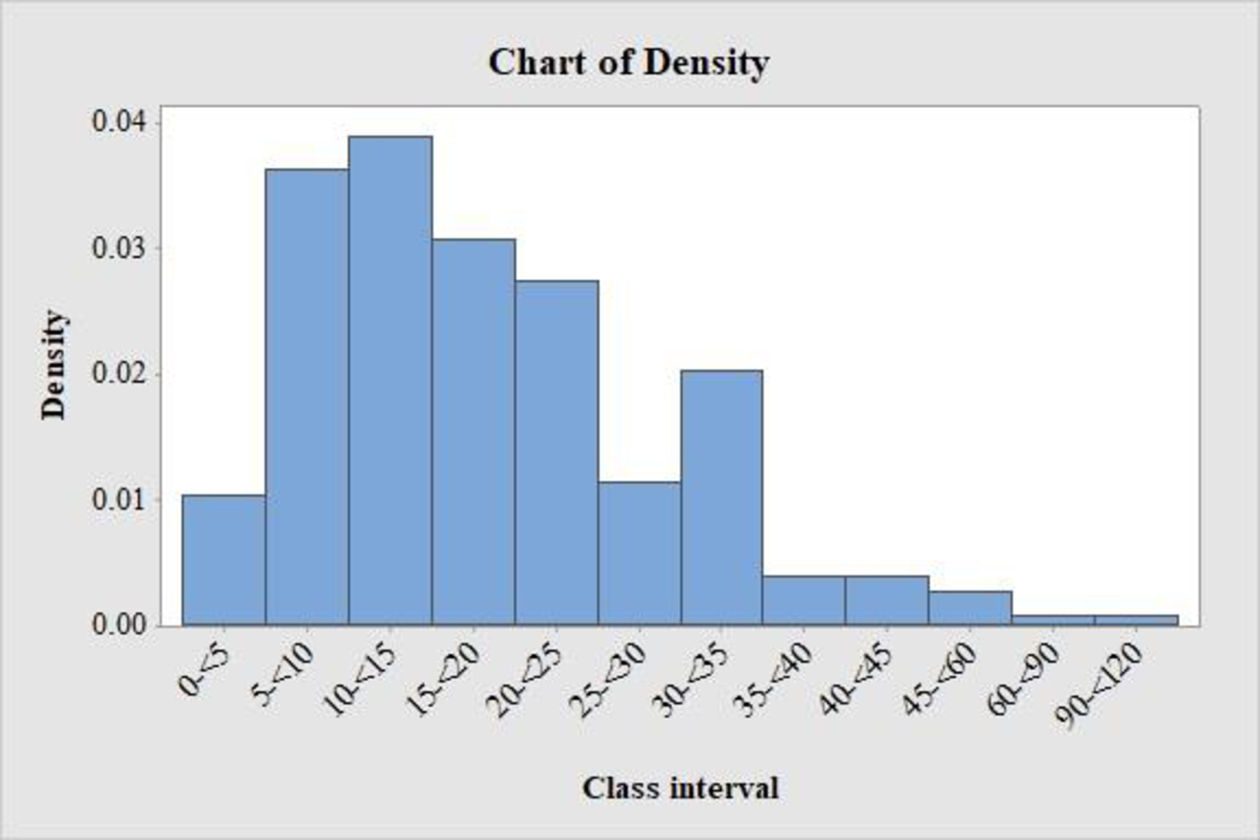
The densities for the class intervals are given below:
| Class interval | Density |
| 0-<5 | 0.0104 |
| 5-<10 | 0.0363 |
| 10-<15 | 0.0390 |
| 15-<20 | 0.0307 |
| 20-<25 | 0.0275 |
| 25-<30 | 0.0114 |
| 30-<35 | 0.0203 |
| 35-<40 | 0.0040 |
| 40-<45 | 0.0040 |
| 45-<60 | 0.0027 |
| 60-<90 | 0.0007 |
| 90-<120 | 0.0007 |
Explanation of Solution
Calculation:
The general formula for the relative frequency is as follows:
Substitute the frequency of the class interval 0-<5 as “5,200” and the total frequency as “100,400” in relative frequency.
Relative frequencies for the remaining class intervals are obtained below:
| Class interval | Frequency | Relative frequency |
| 0-<5 | 5,200 | |
| 5-<10 | 18,200 | |
| 10-<15 | 19,600 | |
| 15-<20 | 15,400 | |
| 20-<25 | 13,800 | |
| 25-<30 | 5,700 | |
| 30-<35 | 10,200 | |
| 35-<40 | 2,000 | |
| 40-<45 | 2,000 | |
| 45-<60 | 4,000 | |
| 60-<90 | 2,100 | |
| 90-<120 | 2,200 | |
| Total | 100,400 |
The general formula for the rectangle height or density is as follows:
Densities of class intervals:
Substitute the relative frequency of the class interval 0-<5 as “0.052”.
Substitute class width as follows:
Density of the class intervals 0-<5 is as follows:
Similarly, densities for the remaining class intervals are obtained below:
| Class interval | Relative frequency | Class width | Density |
| 0-<5 | 0.052 | ||
| 5-<10 | 0.181 | ||
| 10-<15 | 0.195 | ||
| 15-<20 | 0.153 | ||
| 20-<25 | 0.137 | ||
| 25-<30 | 0.057 | ||
| 30-<35 | 0.102 | ||
| 35-<40 | 0.020 | ||
| 40-<45 | 0.020 | ||
| 45-<60 | 0.040 | ||
| 60-<90 | 0.021 | ||
| 90-<120 | 0.022 |
c.
Draw the histogram for the data.
Comment on the important features of the histogram.
c.
Answer to Problem 28E
The histogram is given below:
Explanation of Solution
Calculation:
For the continuous data with unequal class width, the vertical scale of the histogram must be density scale. The rectangle heights are the densities of the intervals.
Here, the class intervals do not have equal length. Hence, the histogram with the relative frequencies is not appropriate.
Therefore, the density of the data has to be used to draw a histogram.
Software procedure:
Step-by-step procedure to draw the histogram using MINITAB software:
- Select Graph > Bar chart.
- In Bars represent select values from a table.
- In one column of values select Simple.
- Enter density in Graph variables.
- Enter Class interval in categorical variable.
- Right click on X-axis; in Edit X Scale in gap between clusters enter 0.
- Select OK.
Observation:
From the histogram, it is observed that the distribution of commute times of working adults is positively skewed with single
The majority of commute times of working adults lies between 5 and 35 minutes.
d.
Find and plot the cumulative frequency distribution for the commute times of working adults.
d.
Answer to Problem 28E
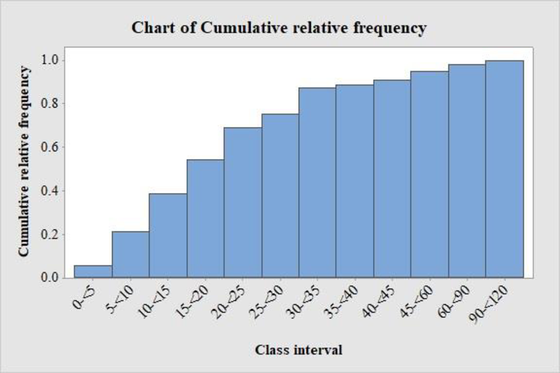
The cumulative relative frequency distribution is as follows:
| Commute time | Cumulative relative frequency |
| 0-<5 | 0.056 |
| 5-<10 | 0.212 |
| 10-<15 | 0.389 |
| 15-<20 | 0.544 |
| 20-<25 | 0.691 |
| 25-<30 | 0.752 |
| 30-<35 | 0.873 |
| 35-<40 | 0.888 |
| 40-<45 | 0.912 |
| 45-<60 | 0.952 |
| 60-<90 | 0.982 |
| 90-<120 | 1 |
The histogram is given below:
Explanation of Solution
Calculation:
Answers may vary; one of the following answers is given below:
Relative frequency distribution:
The general formula for the relative frequency is as follows:
Cumulative relative frequency:
The general formula to obtain cumulative frequency using frequency distribution is as follows:
From the relative frequencies, the cumulative relative frequencies are obtained as follows:
| Commute times | Relative frequency | Cumulative relative frequency |
| 0-<5 | 0.052 | |
| 5-<10 | 0.181 | |
| 10-<15 | 0.195 | |
| 15-<20 | 0.153 | |
| 20-<25 | 0.137 | |
| 25-<30 | 0.057 | |
| 30-<35 | 0.102 | |
| 35-<40 | 0.020 | |
| 40-<45 | 0.020 | |
| 45-<60 | 0.040 | |
| 60-<90 | 0.021 | |
| 90-<120 | 0.022 |
The cumulative relative frequency histogram is plotted for the given data.
Software procedure:
Step-by-step procedure to draw the relative frequency histogram using MINITAB software:
- Select Graph > Bar chart.
- In Bars represent select values from a table.
- In one column of values select Simple.
- Enter Cumulative relative frequency in Graph variables.
- Enter Commute times in categorical variable.
- Right click on X-axis; in Edit X Scale in gap between clusters enter 0.
- Select OK.
e.
(i). Find the approximate proportion of commute times that are less than 50 minutes.
(ii) Find the approximate proportion of commute times that are greater than 22 minutes.
(ii) Find the approximate commute time that separates shortest 50% and longest 50% of commute times.
e.
Answer to Problem 28E
(i) The approximate proportion of commute times that are less than 50 minutes is 0.9253.
(ii) The approximate proportion of commute times that are greater than 22 minutes is 0.3825.
(iii). The commute time that separates shortest 50% and longest 50% of commute times is 30 minutes.
Explanation of Solution
The general formula for the relative frequency or proportion is as follows:
(i). Approximate proportion of commute times that are less than 50 minutes:
The objective is to find the relative frequency of commute times that are less than 50 minutes.
The class width of class interval 45-<60 is 15.
The approximate
The relative frequency of the commute times that are less than 50 minutes is as follows:
Thus, the approximate proportion of commute times are less than 50 minutes is 0.930.
(ii). Approximate proportion of commute times that are greater than 22 minutes:
The objective is to find the relative frequency of commute times that are greater than 22 minutes.
The class width of class interval 20-<25 is 5.
The approximate range of greater than 22 is half of the class interval 20-<25.
Hence, the relative frequency of the commute times that are greater than 22 minutes is as follows:
Thus, the approximate proportion of commute times are greater than 22 minutes is 0.3505.
(iii). Approximate commute time that separates shortest 50% and longest 50% of commute times:
The objective is to find the commute time that separates shortest 50% and longest 50% of commute times.
From the cumulative relative frequency histogram, it is observed that the distribution of commute times of working adults is centered in between 25-<30 and 30-<35 range.
Therefore, the commute time that lies between 25-<30 and 30-<35 range will separate shortest 50% and longest 50% of commute times.
The approximate middle value in between 25-<30 and 30-<35 is 30.
Thus, the approximate commute time that separates shortest 50% and longest 50% of commute times is 30 minutes.
Want to see more full solutions like this?
Chapter 3 Solutions
Introduction to Statistics and Data Analysis


- For a binary asymmetric channel with Py|X(0|1) = 0.1 and Py|X(1|0) = 0.2; PX(0) = 0.4 isthe probability of a bit of “0” being transmitted. X is the transmitted digit, and Y is the received digit.a. Find the values of Py(0) and Py(1).b. What is the probability that only 0s will be received for a sequence of 10 digits transmitted?c. What is the probability that 8 1s and 2 0s will be received for the same sequence of 10 digits?d. What is the probability that at least 5 0s will be received for the same sequence of 10 digits?arrow_forwardV2 360 Step down + I₁ = I2 10KVA 120V 10KVA 1₂ = 360-120 or 2nd Ratio's V₂ m 120 Ratio= 360 √2 H I2 I, + I2 120arrow_forwardQ2. [20 points] An amplitude X of a Gaussian signal x(t) has a mean value of 2 and an RMS value of √(10), i.e. square root of 10. Determine the PDF of x(t).arrow_forward
- In a network with 12 links, one of the links has failed. The failed link is randomlylocated. An electrical engineer tests the links one by one until the failed link is found.a. What is the probability that the engineer will find the failed link in the first test?b. What is the probability that the engineer will find the failed link in five tests?Note: You should assume that for Part b, the five tests are done consecutively.arrow_forwardProblem 3. Pricing a multi-stock option the Margrabe formula The purpose of this problem is to price a swap option in a 2-stock model, similarly as what we did in the example in the lectures. We consider a two-dimensional Brownian motion given by W₁ = (W(¹), W(2)) on a probability space (Q, F,P). Two stock prices are modeled by the following equations: dX = dY₁ = X₁ (rdt+ rdt+0₁dW!) (²)), Y₁ (rdt+dW+0zdW!"), with Xo xo and Yo =yo. This corresponds to the multi-stock model studied in class, but with notation (X+, Y₁) instead of (S(1), S(2)). Given the model above, the measure P is already the risk-neutral measure (Both stocks have rate of return r). We write σ = 0₁+0%. We consider a swap option, which gives you the right, at time T, to exchange one share of X for one share of Y. That is, the option has payoff F=(Yr-XT). (a) We first assume that r = 0 (for questions (a)-(f)). Write an explicit expression for the process Xt. Reminder before proceeding to question (b): Girsanov's theorem…arrow_forwardProblem 1. Multi-stock model We consider a 2-stock model similar to the one studied in class. Namely, we consider = S(1) S(2) = S(¹) exp (σ1B(1) + (M1 - 0/1 ) S(²) exp (02B(2) + (H₂- M2 where (B(¹) ) +20 and (B(2) ) +≥o are two Brownian motions, with t≥0 Cov (B(¹), B(2)) = p min{t, s}. " The purpose of this problem is to prove that there indeed exists a 2-dimensional Brownian motion (W+)+20 (W(1), W(2))+20 such that = S(1) S(2) = = S(¹) exp (011W(¹) + (μ₁ - 01/1) t) 롱) S(²) exp (021W (1) + 022W(2) + (112 - 03/01/12) t). where σ11, 21, 22 are constants to be determined (as functions of σ1, σ2, p). Hint: The constants will follow the formulas developed in the lectures. (a) To show existence of (Ŵ+), first write the expression for both W. (¹) and W (2) functions of (B(1), B(²)). as (b) Using the formulas obtained in (a), show that the process (WA) is actually a 2- dimensional standard Brownian motion (i.e. show that each component is normal, with mean 0, variance t, and that their…arrow_forward
- The scores of 8 students on the midterm exam and final exam were as follows. Student Midterm Final Anderson 98 89 Bailey 88 74 Cruz 87 97 DeSana 85 79 Erickson 85 94 Francis 83 71 Gray 74 98 Harris 70 91 Find the value of the (Spearman's) rank correlation coefficient test statistic that would be used to test the claim of no correlation between midterm score and final exam score. Round your answer to 3 places after the decimal point, if necessary. Test statistic: rs =arrow_forwardBusiness discussarrow_forwardBusiness discussarrow_forward
- I just need to know why this is wrong below: What is the test statistic W? W=5 (incorrect) and What is the p-value of this test? (p-value < 0.001-- incorrect) Use the Wilcoxon signed rank test to test the hypothesis that the median number of pages in the statistics books in the library from which the sample was taken is 400. A sample of 12 statistics books have the following numbers of pages pages 127 217 486 132 397 297 396 327 292 256 358 272 What is the sum of the negative ranks (W-)? 75 What is the sum of the positive ranks (W+)? 5What type of test is this? two tailedWhat is the test statistic W? 5 These are the critical values for a 1-tailed Wilcoxon Signed Rank test for n=12 Alpha Level 0.001 0.005 0.01 0.025 0.05 0.1 0.2 Critical Value 75 70 68 64 60 56 50 What is the p-value for this test? p-value < 0.001arrow_forwardons 12. A sociologist hypothesizes that the crime rate is higher in areas with higher poverty rate and lower median income. She col- lects data on the crime rate (crimes per 100,000 residents), the poverty rate (in %), and the median income (in $1,000s) from 41 New England cities. A portion of the regression results is shown in the following table. Standard Coefficients error t stat p-value Intercept -301.62 549.71 -0.55 0.5864 Poverty 53.16 14.22 3.74 0.0006 Income 4.95 8.26 0.60 0.5526 a. b. Are the signs as expected on the slope coefficients? Predict the crime rate in an area with a poverty rate of 20% and a median income of $50,000. 3. Using data from 50 workarrow_forward2. The owner of several used-car dealerships believes that the selling price of a used car can best be predicted using the car's age. He uses data on the recent selling price (in $) and age of 20 used sedans to estimate Price = Po + B₁Age + ε. A portion of the regression results is shown in the accompanying table. Standard Coefficients Intercept 21187.94 Error 733.42 t Stat p-value 28.89 1.56E-16 Age -1208.25 128.95 -9.37 2.41E-08 a. What is the estimate for B₁? Interpret this value. b. What is the sample regression equation? C. Predict the selling price of a 5-year-old sedan.arrow_forward
 Glencoe Algebra 1, Student Edition, 9780079039897...AlgebraISBN:9780079039897Author:CarterPublisher:McGraw Hill
 Holt Mcdougal Larson Pre-algebra: Student Edition...AlgebraISBN:9780547587776Author:HOLT MCDOUGALPublisher:HOLT MCDOUGAL
 Functions and Change: A Modeling Approach to Coll...AlgebraISBN:9781337111348Author:Bruce Crauder, Benny Evans, Alan NoellPublisher:Cengage Learning
 Algebra: Structure And Method, Book 1AlgebraISBN:9780395977224Author:Richard G. Brown, Mary P. Dolciani, Robert H. Sorgenfrey, William L. ColePublisher:McDougal Littell
 Big Ideas Math A Bridge To Success Algebra 1: Stu...AlgebraISBN:9781680331141Author:HOUGHTON MIFFLIN HARCOURTPublisher:Houghton Mifflin Harcourt