Concept explainers
Videos
The motion picture industry is an extremely competitive business. Dozens of movie studios produce hundreds of movies each year, many of which cost hundreds of millions of dollars to produce and distribute. Some of these movies will go on to earn hundreds of millions of dollars in box office revenues, while others will earn much less than their production cost.
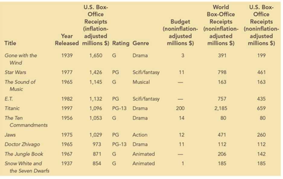
Data from 50 of the top box-office-receipt-generating movies are provided in the file Top50Movies. The following table shows the first 10 movies contained in this data set. The categorical variables included in the data set for each movie are the rating and genre. Quantitative variables for the movie’s release year, inflation- and noninflation-adjusted box-office receipts in the United States, budget, and the world box-office receipts are also included.
Managerial Report
Use the data-visualization methods presented in this chapter to explore these data and discover relationships between the variables. Include the following in your report:
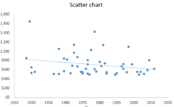
- 1. Create a scatter chart to examine the relationship between the year released and the inflation-adjusted U.S. box office receipts. Include a trendline for this scatter chart. What does the scatter chart indicate about inflation-adjusted U.S. box office receipts over time for these top 50 movies?
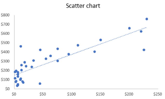
- 2. Create a scatter chart to examine the relationship between the budget and the noninflation-adjusted world box office receipts. (Note: You may have to adjust the data in Excel to ignore the missing budget data values to create your scatter chart. You can do this by first sorting the data using Budget and then creating a scatter chart using only the movies that include data for Budget.) What does this scatter chart indicate about the relationship between the movie’s budget and the world box office receipts?
- 3. Create a frequency distribution, percent frequency distribution, and histogram for inflation-adjusted U.S. box office receipts. Use bin sizes of $100 million. Interpret the results. Do any data points appear to be outliers in this distribution?
- 4. Create a PivotTable for these data. Use the PivotTable to generate a crosstabulation for movie genre and rating. Determine which combinations of genre and rating are most represented in the top 50 movie data. Now filter the data to consider only movies released in 1980 or later. What combinations of genre and rating are most represented for movies after 1980? What does this indicate about how the preferences of moviegoers may have changed over time?
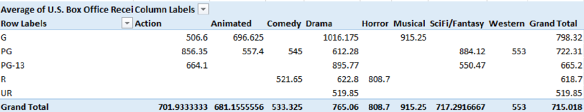
- 5. Use the PivotTable to display the average inflation-adjusted U.S. box-office receipts for each genre–rating pair for all movies in the data set. Interpret the results.
1. Give a scatter chart to examine the relationship between the year released and the inflation-adjusted U.S. box office receipts.
2. Give a scatter chart to examine the relationship between the budget and the noninflation-adjusted world box office receipts.
3. Construct a frequency distribution, percent frequency distribution, and histogram for inflation-adjusted U.S. box office receipts. Give interpretation of the results.
4. Construct crosstabulation for movie genre and rating. Find the combinations of genre and rating that are most represented in the top 50 movie data. Find the combinations of genre that are most represented for movies after 1980.
5. Construct the average inflation-adjusted U.S. box-office receipts for genre-rating pair for all movies in the data set using a PivotTable. Give interpretation.
Answer to Problem 1C
1. The scatter chart of the year released and the inflation-adjusted U.S. box office receipts are as follows:
2. The scatter chart to examine the relationship between the budget and the noninflation-adjusted world box office receipts is as follows:
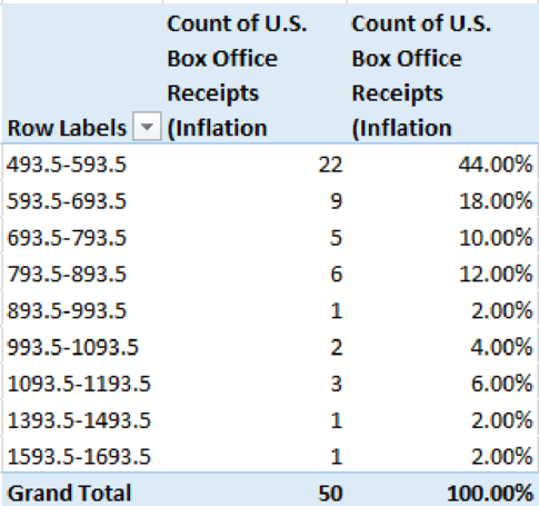
3. The frequency distribution and percent frequency distribution for inflation-adjusted U.S. box office receipts are given below:
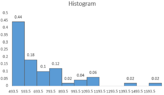
The histogram for inflation-adjusted U.S. box office receipts using an Excel:
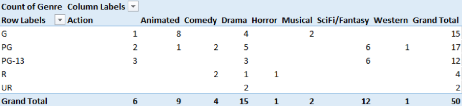
4. The crosstabulation for movie genre and rating for top 50 movies is given below:
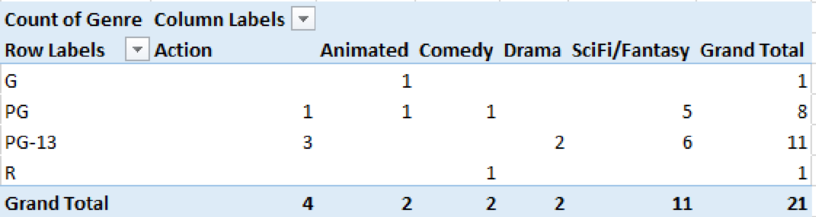
The crosstabulation for movie genre and rating for the movies released after 1980 is as follows:
5. The average inflation-adjusted U.S. box-office receipts for genre-rating pair for all movies in the data set is given below:
Explanation of Solution
1.
Step-by-step procedure to obtain the scatter chart of the year released and the inflation-adjusted U.S. box office receipts using an Excel:
- Select the data of Year Released and U.S. Box Office Receipts (Inflation Adjusted Millions $).
- Select Insert.
- Choose Scatter under Charts.
- In Chart Elements, check Trendline.
Thus, the scatter chart of the year released and the inflation-adjusted U.S. box office receipts is obtained.
From the scatter chart, it is clear that there is slight decrease in inflation over years. However, there is no clear linear pattern observed.
2.
Step-by-step procedure to obtain the scatter chart to examine the relationship between the budget and the noninflation-adjusted world box office receipts using an Excel:
- Select the data of Budget (Non-Inflation Adjusted Millions $) and U.S. Box Office Receipts (Non-Inflation Adjusted Millions $).
- Select Insert.
- Choose Scatter under Charts.
- In Chart Elements, check Trendline.
Thus, the scatter chart to examine the relationship between the budget and the noninflation-adjusted world box office receipts is obtained.
From the output, it is clear that as the budget increases, the noninflation-adjusted world box office receipts also increase.
3.
Step-by-step procedure to create frequency distribution and percent frequency distribution for inflation-adjusted U.S. box office receipts using an Excel:
- Select Insert > PivotTable.
- In Select a table or range, select the data of U.S. Box Office Receipts (Inflation Adjusted Millions $) and click OK.
- In PivotTable Fields, move U.S. Box Office Receipts (Inflation Adjusted Millions $) to Rows and Σ Values.
- Right click on a value from Row Labels.
- Enter 100 in By.
- Click on U.S. Box Office Receipts (Inflation Adjusted Millions $) from Σ Values.
- Select Value Field settings.
- In Summarize value field by, choose Count and click OK.
- Again, move U.S. Box Office Receipts (Inflation Adjusted Millions $) to Rows and Σ Values.
- Click on U.S. Box Office Receipts (Inflation Adjusted Millions $) from Σ Values.
- Select Value Field settings.
- In Show Values As, choose % of Grand Total and click OK.
Thus, the frequency distribution and percent frequency distribution are obtained.
Step-by-step procedure to obtain histogram for inflation-adjusted U.S. box office receipts using an Excel:
- Select the data of class interval and percent frequency.
- Select Insert.
- Choose Clustered Column under Charts.
- Click on a bar in the graph.
- In Format Data Series, enter Gap width as 0%.
Thus, the histogram is obtained.
From the distribution table and histogram, it is clear that the frequency for the lowest inflation-adjusted U.S. box office receipts value is the highest. As the value of inflation-adjusted U.S. box office receipts increases, the frequency decreases. The frequency is very low (2%) for the inflation-adjusted U.S. box office receipts value from 1,393 to 1,593.5. This values seem to be outlier.
4.
Step-by-step procedure to obtain crosstabulation for movie genre and rating for top 50 movies using an Excel:
- Select Insert > PivotTable.
- In Select a table or range, select the data of Rating and Genre and click OK.
- In PivotTable Fields, move Rating to Rows, Genre to Columns, and Genre to Σ Values.
- Click on Genre from Σ Values.
- Select Value Field settings.
- In Summarize value field by, choose Count and click OK.
Thus, the crosstabulation for movie genre and rating for top 50 movies is obtained.
From the crosstabulation of movie genre and rating for top 50 movies, it is observed that the combination of G and Animated (=8) is most represented in the top 50 movie data.
Step-by-step procedure to obtain crosstabulation for movie genre and rating for the movies released after 1980 using an Excel:
- Select the data and choose Filter under Sort & Filter.
- Click on the drop-down box in Year Release column.
- Select Number Filters and choose Greater than.
- In Is greater than, enter 1980.
- Select Insert > PivotTable.
- In Select a table or range, select the filtered data of Rating and Genre and click OK.
- In PivotTable Fields, move Rating to Rows, Genre to Columns, and Genre to Σ Values.
- Click on Genre from Σ Values.
- Select Value Field settings.
- In Summarize value field by, choose Count and click OK.
Thus, the crosstabulation for movie genre and rating for the movies released after 1980 is obtained.
From the crosstabulation of movie genre and rating for the movies released after 1980, it is observed that the combination of PG-13 and SciFi/Fantasy (=6) is most represented.
Also, over the time changes, the number of dramas released became reduced. The rating of G and PG becomes high.
5.
Step-by-step procedure to construct the average inflation-adjusted U.S. box-office receipts for genre-rating pair for all movies in the data set using an Excel:
- Select Insert > PivotTable.
- In Select a table or range, select the filtered data of U.S. Box Office Receipts (Inflation Adjusted Millions $), Rating, and Genre and click OK.
- In PivotTable Fields, move Rating to Rows, Genre to Columns, and U.S. Box Office Receipts (Inflation Adjusted Millions $) to Σ Values.
- Click on Genre from Σ Values.
- Select Value Field settings.
- In Summarize value field by, choose Average and click OK.
Thus, the average inflation-adjusted U.S. box-office receipts for genre-rating pair for all movies in the data set is constructed.
From the table, it is clear that the average U.S. box-office receipts are the highest for the genre-rating pair of G and Drama. Also, it is the lowest for G and Action.
Want to see more full solutions like this?
Chapter 3 Solutions
Mindtap Business Analytics, 1 Term (6 Months) Printed Access Card For Camm/cochran/fry/ohlmann/anderson/sweeney/williams' Essentials Of Business Analytics, 2nd


- A television news channel samples 25 gas stations from its local area and uses the results to estimate the average gas price for the state. What’s wrong with its margin of error?arrow_forwardYou’re fed up with keeping Fido locked inside, so you conduct a mail survey to find out people’s opinions on the new dog barking ordinance in a certain city. Of the 10,000 people who receive surveys, 1,000 respond, and only 80 are in favor of it. You calculate the margin of error to be 1.2 percent. Explain why this reported margin of error is misleading.arrow_forwardYou find out that the dietary scale you use each day is off by a factor of 2 ounces (over — at least that’s what you say!). The margin of error for your scale was plus or minus 0.5 ounces before you found this out. What’s the margin of error now?arrow_forward
- Suppose that Sue and Bill each make a confidence interval out of the same data set, but Sue wants a confidence level of 80 percent compared to Bill’s 90 percent. How do their margins of error compare?arrow_forwardSuppose that you conduct a study twice, and the second time you use four times as many people as you did the first time. How does the change affect your margin of error? (Assume the other components remain constant.)arrow_forwardOut of a sample of 200 babysitters, 70 percent are girls, and 30 percent are guys. What’s the margin of error for the percentage of female babysitters? Assume 95 percent confidence.What’s the margin of error for the percentage of male babysitters? Assume 95 percent confidence.arrow_forward
- You sample 100 fish in Pond A at the fish hatchery and find that they average 5.5 inches with a standard deviation of 1 inch. Your sample of 100 fish from Pond B has the same mean, but the standard deviation is 2 inches. How do the margins of error compare? (Assume the confidence levels are the same.)arrow_forwardA survey of 1,000 dental patients produces 450 people who floss their teeth adequately. What’s the margin of error for this result? Assume 90 percent confidence.arrow_forwardThe annual aggregate claim amount of an insurer follows a compound Poisson distribution with parameter 1,000. Individual claim amounts follow a Gamma distribution with shape parameter a = 750 and rate parameter λ = 0.25. 1. Generate 20,000 simulated aggregate claim values for the insurer, using a random number generator seed of 955.Display the first five simulated claim values in your answer script using the R function head(). 2. Plot the empirical density function of the simulated aggregate claim values from Question 1, setting the x-axis range from 2,600,000 to 3,300,000 and the y-axis range from 0 to 0.0000045. 3. Suggest a suitable distribution, including its parameters, that approximates the simulated aggregate claim values from Question 1. 4. Generate 20,000 values from your suggested distribution in Question 3 using a random number generator seed of 955. Use the R function head() to display the first five generated values in your answer script. 5. Plot the empirical density…arrow_forward
- Find binomial probability if: x = 8, n = 10, p = 0.7 x= 3, n=5, p = 0.3 x = 4, n=7, p = 0.6 Quality Control: A factory produces light bulbs with a 2% defect rate. If a random sample of 20 bulbs is tested, what is the probability that exactly 2 bulbs are defective? (hint: p=2% or 0.02; x =2, n=20; use the same logic for the following problems) Marketing Campaign: A marketing company sends out 1,000 promotional emails. The probability of any email being opened is 0.15. What is the probability that exactly 150 emails will be opened? (hint: total emails or n=1000, x =150) Customer Satisfaction: A survey shows that 70% of customers are satisfied with a new product. Out of 10 randomly selected customers, what is the probability that at least 8 are satisfied? (hint: One of the keyword in this question is “at least 8”, it is not “exactly 8”, the correct formula for this should be = 1- (binom.dist(7, 10, 0.7, TRUE)). The part in the princess will give you the probability of seven and less than…arrow_forwardplease answer these questionsarrow_forwardSelon une économiste d’une société financière, les dépenses moyennes pour « meubles et appareils de maison » ont été moins importantes pour les ménages de la région de Montréal, que celles de la région de Québec. Un échantillon aléatoire de 14 ménages pour la région de Montréal et de 16 ménages pour la région Québec est tiré et donne les données suivantes, en ce qui a trait aux dépenses pour ce secteur d’activité économique. On suppose que les données de chaque population sont distribuées selon une loi normale. Nous sommes intéressé à connaitre si les variances des populations sont égales.a) Faites le test d’hypothèse sur deux variances approprié au seuil de signification de 1 %. Inclure les informations suivantes : i. Hypothèse / Identification des populationsii. Valeur(s) critique(s) de Fiii. Règle de décisioniv. Valeur du rapport Fv. Décision et conclusion b) A partir des résultats obtenus en a), est-ce que l’hypothèse d’égalité des variances pour cette…arrow_forward
 Glencoe Algebra 1, Student Edition, 9780079039897...AlgebraISBN:9780079039897Author:CarterPublisher:McGraw Hill
 Elementary Geometry for College StudentsGeometryISBN:9781285195698Author:Daniel C. Alexander, Geralyn M. KoeberleinPublisher:Cengage Learning
 Holt Mcdougal Larson Pre-algebra: Student Edition...AlgebraISBN:9780547587776Author:HOLT MCDOUGALPublisher:HOLT MCDOUGAL
 Functions and Change: A Modeling Approach to Coll...AlgebraISBN:9781337111348Author:Bruce Crauder, Benny Evans, Alan NoellPublisher:Cengage Learning