Connect Hosted by ALEKS Access Card or Elementary Statistics
3rd Edition
ISBN: 9781260373752
Author: William Navidi Prof., Barry Monk Professor
Publisher: McGraw-Hill Education
expand_more
expand_more
format_list_bulleted
Concept explainers
Videos
Textbook Question
Chapter 2.3, Problem 32E
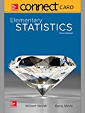
More gold: The following time series plot presents the number of countries participating in the Summer Olympic games in each Olympic year from 1952 through 2016.
Refer to Exercise 30. Someone says “Although the number of gold medals won by the United States didn’t change much from 1952 to 1972, the performance of the United States steadily improved during that period.” Which feature of the plot of the number of participating countries justifies that statement?
Expert Solution & Answer
Want to see the full answer?
Check out a sample textbook solution
Students have asked these similar questions
I need help with this problem and an explanation of the solution for the image described below. (Statistics: Engineering Probabilities)
I need help with this problem and an explanation of the solution for the image described below. (Statistics: Engineering Probabilities)
310015
K
Question 9,
5.2.28-T
Part 1 of 4
HW Score:
85.96%, 49 of
57 points
Points: 1
Save
of 6
Based on a poll, among adults who regret getting tattoos, 28%
say that they were too young when they got their tattoos.
Assume that six adults who regret getting tattoos are
randomly selected, and find the indicated probability. Complete
parts (a) through (d) below.
a. Find the probability that none of the selected adults say that
they were too young to get tattoos.
0.0520 (Round to four decimal places as needed.)
Clear all
Final check
Feb 7 12:47 US O
Chapter 2 Solutions
Connect Hosted by ALEKS Access Card or Elementary Statistics
Ch. 2.1 - In Exercises 5-8, fill in each blank with the...Ch. 2.1 - In Exercises 5-8, fill in each blank with the...Ch. 2.1 - In Exercises 5-8, fill in each blank with the...Ch. 2.1 - In Exercises 5-8, fill in each blank with the...Ch. 2.1 - In Exercises 9—12, determine whether the...Ch. 2.1 - In Exercises 9—12, determine whether the...Ch. 2.1 - In Exercises 9—12, determine whether the...Ch. 2.1 - In Exercises 9—12, determine whether the...Ch. 2.1 - The following bar graph presents the average...Ch. 2.1 - The most common blood typing system divides human...
Ch. 2.1 - Following is a pie chart that presents the...Ch. 2.1 - Government spending: The following pie chart...Ch. 2.1 - U.S. population: The following side-by-side bar...Ch. 2.1 - Super Bowl: The following side-by-side bar graph...Ch. 2.1 - Smartphone sales: The following frequency...Ch. 2.1 - Popular video games: The following frequency...Ch. 2.1 - More smartphones: Using the data in Exercise 19:...Ch. 2.1 - More video games: Using the data in Exercise 20:...Ch. 2.1 - Hospital admissions: The following frequency...Ch. 2.1 - World population: Following are the populations of...Ch. 2.1 - Ages of video garners: The Nielsen Company...Ch. 2.1 - How secure is your job? In a survey, employed...Ch. 2.1 - Back up your data: In a survey commissioned by the...Ch. 2.1 - Education levels: The following frequency...Ch. 2.1 - Twitter followers: The following frequency...Ch. 2.1 - Music sales: The following frequency distribution...Ch. 2.1 - Keeping up with the Kardashians: The following...Ch. 2.1 - Bought a new car lately? The following table...Ch. 2.1 - Bought a new- truck lately? The following table...Ch. 2.1 - Happy Halloween: The following table presents...Ch. 2.1 - Native languages: The following frequency...Ch. 2.1 - Proportion of females: Following are the...Ch. 2.2 - Prob. 5ECh. 2.2 - In Exercises 5—8, fill in each blank with the...Ch. 2.2 - In Exercises 5—8, fill in each blank with the...Ch. 2.2 - In Exercises 5—8, fill in each blank with the...Ch. 2.2 - In Exercises 9—12, determine whether the...Ch. 2.2 - In Exercises 9—12, determine whether the...Ch. 2.2 - In Exercises 9—12, determine whether the...Ch. 2.2 - In Exercises 9—12, determine whether the...Ch. 2.2 - In Exercises 13—16, classify the histogram as...Ch. 2.2 - In Exercises 13—16, classify the histogram as...Ch. 2.2 - In Exercises 13—16, classify the histogram as...Ch. 2.2 - In Exercises 13—16, classify the histogram as...Ch. 2.2 - In Exercises 17 and 18, classify the histogram as...Ch. 2.2 - In Exercises 17 and 18, classify the histogram as...Ch. 2.2 - Student heights: The following frequency histogram...Ch. 2.2 - Trained rats: Forty rats were trained to run a...Ch. 2.2 - Cholesterol: The following histogram shows the...Ch. 2.2 - Blood pressure: The following histogram shows the...Ch. 2.2 - Olympic athletes: The following frequency...Ch. 2.2 - Hows the weather? The following relative frequency...Ch. 2.2 - Skewed which way? For which of the following data...Ch. 2.2 - Skewed which way? For which of the following data...Ch. 2.2 - Batting average: The following frequency...Ch. 2.2 - Batting average: The following frequency...Ch. 2.2 - Time spent playing video games: A sample of 200...Ch. 2.2 - Murder, she wrote: The following frequency...Ch. 2.2 - BMW prices: The following table presents the...Ch. 2.2 - Geysers: The geyser Old Faithful in Yellowstone...Ch. 2.2 - Hail to the chief: There have been 58 presidential...Ch. 2.2 - Internet radio: The following table presents the...Ch. 2.2 - Brothers and sisters: Thirty students in a...Ch. 2.2 - Cough, cough: The following table presents the...Ch. 2.2 - Prob. 37ECh. 2.2 - Prob. 38ECh. 2.2 - Prob. 39ECh. 2.2 - Prob. 40ECh. 2.2 - Frequency polygon: Using the data in Exercise 29:...Ch. 2.2 - Prob. 42ECh. 2.2 - Ogive: Using the data in Exercise 27: Compute the...Ch. 2.2 - Ogive: Using the data in Exercise 28: Compute the...Ch. 2.2 - Ogive: Using the data in Exercise 29: Compute the...Ch. 2.2 - Prob. 46ECh. 2.2 - Prob. 47ECh. 2.2 - Prob. 48ECh. 2.2 - Prob. 49ECh. 2.2 - Prob. 50ECh. 2.2 - Prob. 51ECh. 2.2 - Prob. 52ECh. 2.2 - Frequencies and relative frequencies: The...Ch. 2.3 - In Exercises 3—6, fill in each blank with the...Ch. 2.3 - In Exercises 3—6, fill in each blank with the...Ch. 2.3 - In Exercises 3—6, fill in each blank with the...Ch. 2.3 - In Exercises 3—6, fill in each blank with the...Ch. 2.3 - Prob. 7ECh. 2.3 - In Exercises 7—10, determine whether the...Ch. 2.3 - In Exercises 7—10, determine whether the...Ch. 2.3 - In Exercises 7—10, determine whether the...Ch. 2.3 - Construct a stem-and-leaf plot for the following...Ch. 2.3 - Construct a stem-and-leaf plot for the following...Ch. 2.3 - List the data in the following stem-and-leaf plot....Ch. 2.3 - List the data in the following stein-and-leaf...Ch. 2.3 - Construct a dotplot for the data in Exercise 11.Ch. 2.3 - Prob. 16ECh. 2.3 - BMW prices: The following table presents the...Ch. 2.3 - Hows the weather? The following table presents the...Ch. 2.3 - Air pollution: The following table presents...Ch. 2.3 - Technology salaries: The following table presents...Ch. 2.3 - Tennis and golf: Following are the ages of the...Ch. 2.3 - Pass the popcorn: Following are the running times...Ch. 2.3 - More weather: Construct a dotplot for the data in...Ch. 2.3 - Prob. 24ECh. 2.3 - Looking for a job: The following table presents...Ch. 2.3 - Prob. 26ECh. 2.3 - Military spending: The following table presents...Ch. 2.3 - Prob. 28ECh. 2.3 - Dining out: The following time-series plot...Ch. 2.3 - Prob. 30ECh. 2.3 - Prob. 31ECh. 2.3 - More gold: The following time series plot presents...Ch. 2.3 - Prob. 33ECh. 2.3 - Prob. 34ECh. 2.3 - Vote: The following time-series plot presents the...Ch. 2.3 - Arctic ice sheet: The following table presents the...Ch. 2.3 - Prob. 37ECh. 2.4 - In Exercises 3 and 4, fill in each blank with the...Ch. 2.4 - In Exercises 3 and 4, fill in each blank with the...Ch. 2.4 - CD sales decline: Sales of CDs have been declining...Ch. 2.4 - Music sales: The following time-series plot and...Ch. 2.4 - Stock market prices: The Dow Jones Industrial...Ch. 2.4 - Save your money: In 2007, U.S. residents saved...Ch. 2.4 - Ill take mine with mustard: The following bar...Ch. 2.4 - Stream or download? The following bar graph...Ch. 2.4 - Female senators: Of the 100 members of the United...Ch. 2.4 - Age at marriage: Data compiled by the U.S. Census...Ch. 2.4 - College degrees: Both of the following time-series...Ch. 2.4 - Food expenditures: Both of the following...Ch. 2.4 - Prob. 15ECh. 2 - Following is the list of letter grades for...Ch. 2 - Prob. 2CQCh. 2 - Construct a frequency bar graph for the data in...Ch. 2 - Prob. 4CQCh. 2 - Prob. 5CQCh. 2 - Prob. 6CQCh. 2 - Prob. 7CQCh. 2 - Prob. 8CQCh. 2 - Prob. 9CQCh. 2 - Prob. 10CQCh. 2 - Following are the prices (in dollars) for a sample...Ch. 2 - Prob. 12CQCh. 2 - Prob. 13CQCh. 2 - Prob. 14CQCh. 2 - Prob. 15CQCh. 2 - Trust your doctor: The General Social Survey...Ch. 2 - Internet browsers: The following relative...Ch. 2 - Prob. 3RECh. 2 - Prob. 4RECh. 2 - Prob. 5RECh. 2 - House freshmen: Newly elected members of the U.S....Ch. 2 - More freshmen: For the data in Exercise 6:...Ch. 2 - Royalty: Following are the ages at death for all...Ch. 2 - Prob. 9RECh. 2 - Prob. 10RECh. 2 - Prob. 11RECh. 2 - Prob. 12RECh. 2 - Prob. 13RECh. 2 - Prob. 14RECh. 2 - Prob. 15RECh. 2 - Explain why the frequency bar graph and the...Ch. 2 - Prob. 2WAICh. 2 - Prob. 3WAICh. 2 - Prob. 4WAICh. 2 - Prob. 5WAICh. 2 - In the chapter introduction, we presented gas...Ch. 2 - In the chapter introduction, we presented gas...Ch. 2 - In the chapter introduction, we presented gas...Ch. 2 - Prob. 4CSCh. 2 - In the chapter introduction, we presented gas...Ch. 2 - Prob. 6CSCh. 2 - In the chapter introduction, we presented gas...Ch. 2 - Prob. 8CSCh. 2 - In the chapter introduction, we presented gas...
Knowledge Booster


Learn more about
Need a deep-dive on the concept behind this application? Look no further. Learn more about this topic, statistics and related others by exploring similar questions and additional content below.Similar questions
- how could the bar graph have been organized differently to make it easier to compare opinion changes within political partiesarrow_forwardDraw a picture of a normal distribution with mean 70 and standard deviation 5.arrow_forwardWhat do you guess are the standard deviations of the two distributions in the previous example problem?arrow_forward
- Please answer the questionsarrow_forward30. An individual who has automobile insurance from a certain company is randomly selected. Let Y be the num- ber of moving violations for which the individual was cited during the last 3 years. The pmf of Y isy | 1 2 4 8 16p(y) | .05 .10 .35 .40 .10 a.Compute E(Y).b. Suppose an individual with Y violations incurs a surcharge of $100Y^2. Calculate the expected amount of the surcharge.arrow_forward24. An insurance company offers its policyholders a num- ber of different premium payment options. For a ran- domly selected policyholder, let X = the number of months between successive payments. The cdf of X is as follows: F(x)=0.00 : x < 10.30 : 1≤x<30.40 : 3≤ x < 40.45 : 4≤ x <60.60 : 6≤ x < 121.00 : 12≤ x a. What is the pmf of X?b. Using just the cdf, compute P(3≤ X ≤6) and P(4≤ X).arrow_forward
- 59. At a certain gas station, 40% of the customers use regular gas (A1), 35% use plus gas (A2), and 25% use premium (A3). Of those customers using regular gas, only 30% fill their tanks (event B). Of those customers using plus, 60% fill their tanks, whereas of those using premium, 50% fill their tanks.a. What is the probability that the next customer will request plus gas and fill the tank (A2 B)?b. What is the probability that the next customer fills the tank?c. If the next customer fills the tank, what is the probability that regular gas is requested? Plus? Premium?arrow_forward38. Possible values of X, the number of components in a system submitted for repair that must be replaced, are 1, 2, 3, and 4 with corresponding probabilities .15, .35, .35, and .15, respectively. a. Calculate E(X) and then E(5 - X).b. Would the repair facility be better off charging a flat fee of $75 or else the amount $[150/(5 - X)]? [Note: It is not generally true that E(c/Y) = c/E(Y).]arrow_forward74. The proportions of blood phenotypes in the U.S. popula- tion are as follows:A B AB O .40 .11 .04 .45 Assuming that the phenotypes of two randomly selected individuals are independent of one another, what is the probability that both phenotypes are O? What is the probability that the phenotypes of two randomly selected individuals match?arrow_forward
- 53. A certain shop repairs both audio and video compo- nents. Let A denote the event that the next component brought in for repair is an audio component, and let B be the event that the next component is a compact disc player (so the event B is contained in A). Suppose that P(A) = .6 and P(B) = .05. What is P(BA)?arrow_forward26. A certain system can experience three different types of defects. Let A;(i = 1,2,3) denote the event that the sys- tem has a defect of type i. Suppose thatP(A1) = .12 P(A) = .07 P(A) = .05P(A, U A2) = .13P(A, U A3) = .14P(A2 U A3) = .10P(A, A2 A3) = .011Rshelfa. What is the probability that the system does not havea type 1 defect?b. What is the probability that the system has both type 1 and type 2 defects?c. What is the probability that the system has both type 1 and type 2 defects but not a type 3 defect? d. What is the probability that the system has at most two of these defects?arrow_forwardThe following are suggested designs for group sequential studies. Using PROCSEQDESIGN, provide the following for the design O’Brien Fleming and Pocock.• The critical boundary values for each analysis of the data• The expected sample sizes at each interim analysisAssume the standardized Z score method for calculating boundaries.Investigators are evaluating the success rate of a novel drug for treating a certain type ofbacterial wound infection. Since no existing treatment exists, they have planned a one-armstudy. They wish to test whether the success rate of the drug is better than 50%, whichthey have defined as the null success rate. Preliminary testing has estimated the successrate of the drug at 55%. The investigators are eager to get the drug into production andwould like to plan for 9 interim analyses (10 analyzes in total) of the data. Assume thesignificance level is 5% and power is 90%.Besides, draw a combined boundary plot (OBF, POC, and HP)arrow_forward
arrow_back_ios
SEE MORE QUESTIONS
arrow_forward_ios
Recommended textbooks for you
 MATLAB: An Introduction with ApplicationsStatisticsISBN:9781119256830Author:Amos GilatPublisher:John Wiley & Sons Inc
 Probability and Statistics for Engineering and th...StatisticsISBN:9781305251809Author:Jay L. DevorePublisher:Cengage Learning
 Statistics for The Behavioral Sciences (MindTap C...StatisticsISBN:9781305504912Author:Frederick J Gravetter, Larry B. WallnauPublisher:Cengage Learning
 Elementary Statistics: Picturing the World (7th E...StatisticsISBN:9780134683416Author:Ron Larson, Betsy FarberPublisher:PEARSON
 The Basic Practice of StatisticsStatisticsISBN:9781319042578Author:David S. Moore, William I. Notz, Michael A. FlignerPublisher:W. H. Freeman
 Introduction to the Practice of StatisticsStatisticsISBN:9781319013387Author:David S. Moore, George P. McCabe, Bruce A. CraigPublisher:W. H. Freeman
MATLAB: An Introduction with Applications
Statistics
ISBN:9781119256830
Author:Amos Gilat
Publisher:John Wiley & Sons Inc
Probability and Statistics for Engineering and th...
Statistics
ISBN:9781305251809
Author:Jay L. Devore
Publisher:Cengage Learning
Statistics for The Behavioral Sciences (MindTap C...
Statistics
ISBN:9781305504912
Author:Frederick J Gravetter, Larry B. Wallnau
Publisher:Cengage Learning
Elementary Statistics: Picturing the World (7th E...
Statistics
ISBN:9780134683416
Author:Ron Larson, Betsy Farber
Publisher:PEARSON
The Basic Practice of Statistics
Statistics
ISBN:9781319042578
Author:David S. Moore, William I. Notz, Michael A. Fligner
Publisher:W. H. Freeman
Introduction to the Practice of Statistics
Statistics
ISBN:9781319013387
Author:David S. Moore, George P. McCabe, Bruce A. Craig
Publisher:W. H. Freeman
Correlation Vs Regression: Difference Between them with definition & Comparison Chart; Author: Key Differences;https://www.youtube.com/watch?v=Ou2QGSJVd0U;License: Standard YouTube License, CC-BY
Correlation and Regression: Concepts with Illustrative examples; Author: LEARN & APPLY : Lean and Six Sigma;https://www.youtube.com/watch?v=xTpHD5WLuoA;License: Standard YouTube License, CC-BY