Videos
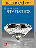
Education levels: The following frequency distribution categorizes US. adults aged 18 and over by educational attainment in a recent year.
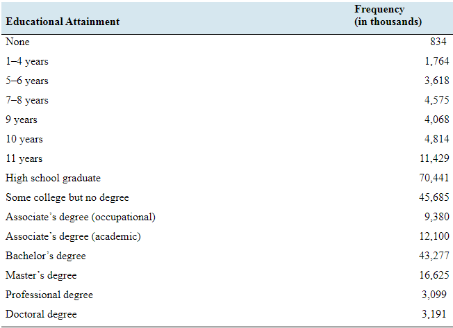
- Construct a frequency bar graph.
- Construct a relative frequency distribution.
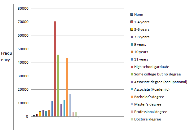
- Construct a relative frequency bar graph.
- Construct a frequency distribution with the following categories: 8 years or less, 9—11 years, High school graduate, Some college but no degree: College degree (Associate’s or Bachelor’s): Graduate degree Master’s, Professional, or Doctoral).
- Construct a pie chart for the frequency distribution in part (d).
- What proportion of people did not graduate from high school?
a.
To construct: A frequency bar graph.
Explanation of Solution
Given information: The following frequency distribution categorises U.S. adults aged 18 and over by educational attainment in a recent year.
| Educational attainment | Frequency(in thousands) |
| None | 834 |
| 1-4 years | 1764 |
| 5-6 years | 3618 |
| 7-8 years | 4575 |
| 9 years | 4068 |
| 10 years | 4814 |
| 11 years | 11429 |
| High school graduate | 70441 |
| Some college but no degree | 45685 |
| Associates degree (Occupational) | 9380 |
| Associates degree (Academic) | 12100 |
| Bachelor’s degree | 43277 |
| Master’s degree | 16625 |
| Professional degree | 3099 |
| Doctoral degree | 3191 |
Solution:
From the given table, the frequency bar graph is given by
b.
To construct: The relative frequency distribution.
Explanation of Solution
Given information:The following frequency distribution categorises U.S. adults aged 18 and over by educational attainment in a recent year.
| Educational attainment | Frequency(in thousands) |
| None | 834 |
| 1-4 years | 1764 |
| 5-6 years | 3618 |
| 7-8 years | 4575 |
| 9 years | 4068 |
| 10 years | 4814 |
| 11 years | 11429 |
| High school graduate | 70441 |
| Some college but no degree | 45685 |
| Associates degree (Occupational) | 9380 |
| Associates degree (Academic) | 12100 |
| Bachelor’s degree | 43277 |
| Master’s degree | 16625 |
| Professional degree | 3099 |
| Doctoral degree | 3191 |
Formula used:
Calculation:
From the given table,
The sum of all frequency is
The table of relative frequency is given by
| Educational attainment | Frequency(in thousands) | Relative frequency |
| None | 834 | |
| 1-4 years | 1764 | |
| 5-6 years | 3618 | |
| 7-8 years | 4575 | |
| 9 years | 4068 | |
| 10 years | 4814 | |
| 11 years | 11429 | |
| High school graduate | 70441 | |
| Some college but no degree | 45685 | |
| Associates degree (Occupational) | 9380 | |
| Associates degree (Academic) | 12100 | |
| Bachelor’s degree | 43277 | |
| Master’s degree | 16625 | |
| Professional degree | 3099 | |
| Doctoral degree | 3191 |
c.
To construct: A relative frequency bar graph.
Explanation of Solution
Given information:The following frequency distribution categorises U.S. adults aged 18 and over by educational attainment in a recent year.
| Educational attainment | Frequency(in thousands) |
| None | 834 |
| 1-4 years | 1764 |
| 5-6 years | 3618 |
| 7-8 years | 4575 |
| 9 years | 4068 |
| 10 years | 4814 |
| 11 years | 11429 |
| High school graduate | 70441 |
| Some college but no degree | 45685 |
| Associates degree (Occupational) | 9380 |
| Associates degree (Academic) | 12100 |
| Bachelor’s degree | 43277 |
| Master’s degree | 16625 |
| Professional degree | 3099 |
| Doctoral degree | 3191 |
Definition used:
Histogram based on relative frequency is called relative frequency histogram.
Solution:
The following table gives the relative frequency.
| Educational attainment | Relative frequency |
| None | 0.0036 |
| 1-4 years | 0.0075 |
| 5-6 years | 0.0154 |
| 7-8 years | 0.0195 |
| 9 years | 0.0173 |
| 10 years | 0.0205 |
| 11 years | 0.0487 |
| High school graduate | 0.2999 |
| Some college but no degree | 0.1945 |
| Associates degree (Occupational) | 0.0399 |
| Associates degree (Academic) | 0.0515 |
| Bachelor’s degree | 0.184 |
| Master’s degree | 0.0708 |
| Professional degree | 0.0132 |
| Doctoral degree | 0.0136 |
From the above table, the relative frequency bar graph is given by
d.
To construct: A frequency distribution with the following categories: 8 years or less, 9-11 years, High school graduate, Some college but no degree, College degree (Associate’s or Bachelor’s), Graduate degree (Master’s, professional, or Doctoral)
Answer to Problem 28E
| Educational attainment | Frequency(in thousands) |
| 8 years or less | 10791 |
| 9-11 years | 20311 |
| High school graduate | 70441 |
| Some college but no degree | 45685 |
| College degree (Associate’s or Bachelor’s) | 64757 |
| Graduate degree (Master’s, professional, or Doctoral) | 22915 |
Explanation of Solution
Given information:The following frequency distribution categorises U.S. adults aged 18 and over by educational attainment in a recent year.
| Educational attainment | Frequency(in thousands) |
| None | 834 |
| 1-4 years | 1764 |
| 5-6 years | 3618 |
| 7-8 years | 4575 |
| 9 years | 4068 |
| 10 years | 4814 |
| 11 years | 11429 |
| High school graduate | 70441 |
| Some college but no degree | 45685 |
| Associates degree (Occupational) | 9380 |
| Associates degree (Academic) | 12100 |
| Bachelor’s degree | 43277 |
| Master’s degree | 16625 |
| Professional degree | 3099 |
| Doctoral degree | 3191 |
Solution:
The required frequency distribution with the given categories is given by
| Educational attainment | Frequency(in thousands) |
| 8 years or less | |
| 9-11 years | |
| High school graduate | 70441 |
| Some college but no degree | 45685 |
| College degree (Associate’s or Bachelor’s) | |
| Graduate degree (Master’s, professional, or Doctoral) |
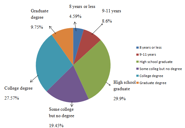
e.
To construct: A pie chart
Explanation of Solution
Given information: The following frequency distribution categorises U.S. adults aged 18 and over by educational attainment in a recent year.
| Educational attainment | Frequency(in thousands) |
| 8 years or less | 10791 |
| 9-11 years | 20311 |
| High school graduate | 70441 |
| Some college but no degree | 45685 |
| College degree (Associate’s or Bachelor’s) | 64757 |
| Graduate degree (Master’s, professional, or Doctoral) | 22915 |
Solution:
From the given table, the percentage of each gender and age group is given by
| Educational attainment | Frequency(in thousands) | Relative frequency | Percentage |
| 8 years or less | 10791 | 0.0459 | 4.59 % |
| 9-11 years | 10311 | 0.086 | 8.6% |
| High school graduate | 70441 | 0.299 | 29.9% |
| Some college but no degree | 45685 | 0.1945 | 19.45% |
| College degree (Associate’s or Bachelor’s) | 64757 | 0.2757 | 27.57% |
| Graduate degree (Master’s, professional, or Doctoral) | 22915 | 0.0975 | 9.75% |
From the above table, the pie chart is given by
f.
To find: The proportion of people did not graduate from high school.
Answer to Problem 28E
The proportion of people did not graduate from high school is 0.132.
Explanation of Solution
Given information:The following frequency distribution categorises U.S. adults aged 18 and over by educational attainment in a recent year.
| Educational attainment | Frequency(in thousands) |
| 8 years or less | 10791 |
| 9-11 years | 20311 |
| High school graduate | 70441 |
| Some college but no degree | 45685 |
| College degree (Associate’s or Bachelor’s) | 64757 |
| Graduate degree (Master’s, professional, or Doctoral) | 22915 |
Solution:
From the given table, the percentage of each gender and age group is given by
| Educational attainment | Frequency(in thousands) | Relative frequency |
| 8 years or less | 10791 | 0.0459 |
| 9-11 years | 20311 | 0.086 |
| High school graduate | 70441 | 0.299 |
| Some college but no degree | 45685 | 0.1945 |
| College degree (Associate’s or Bachelor’s) | 64757 | 0.2757 |
| Graduate degree (Master’s, professional, or Doctoral) | 22915 | 0.0975 |
The people did not graduate from high school are people whose educations are 8 years or less and 9-11 years.
The proportion of people did not graduate from high school is
Hence, the proportion of people did not graduate from high school is 0.132.
Want to see more full solutions like this?
Chapter 2 Solutions
Connect Hosted by ALEKS Access Card or Elementary Statistics


- step by step on Microssoft on how to put this in excel and the answers please Find binomial probability if: x = 8, n = 10, p = 0.7 x= 3, n=5, p = 0.3 x = 4, n=7, p = 0.6 Quality Control: A factory produces light bulbs with a 2% defect rate. If a random sample of 20 bulbs is tested, what is the probability that exactly 2 bulbs are defective? (hint: p=2% or 0.02; x =2, n=20; use the same logic for the following problems) Marketing Campaign: A marketing company sends out 1,000 promotional emails. The probability of any email being opened is 0.15. What is the probability that exactly 150 emails will be opened? (hint: total emails or n=1000, x =150) Customer Satisfaction: A survey shows that 70% of customers are satisfied with a new product. Out of 10 randomly selected customers, what is the probability that at least 8 are satisfied? (hint: One of the keyword in this question is “at least 8”, it is not “exactly 8”, the correct formula for this should be = 1- (binom.dist(7, 10, 0.7,…arrow_forwardKate, Luke, Mary and Nancy are sharing a cake. The cake had previously been divided into four slices (s1, s2, s3 and s4). What is an example of fair division of the cake S1 S2 S3 S4 Kate $4.00 $6.00 $6.00 $4.00 Luke $5.30 $5.00 $5.25 $5.45 Mary $4.25 $4.50 $3.50 $3.75 Nancy $6.00 $4.00 $4.00 $6.00arrow_forwardFaye cuts the sandwich in two fair shares to her. What is the first half s1arrow_forward
- Question 2. An American option on a stock has payoff given by F = f(St) when it is exercised at time t. We know that the function f is convex. A person claims that because of convexity, it is optimal to exercise at expiration T. Do you agree with them?arrow_forwardQuestion 4. We consider a CRR model with So == 5 and up and down factors u = 1.03 and d = 0.96. We consider the interest rate r = 4% (over one period). Is this a suitable CRR model? (Explain your answer.)arrow_forwardQuestion 3. We want to price a put option with strike price K and expiration T. Two financial advisors estimate the parameters with two different statistical methods: they obtain the same return rate μ, the same volatility σ, but the first advisor has interest r₁ and the second advisor has interest rate r2 (r1>r2). They both use a CRR model with the same number of periods to price the option. Which advisor will get the larger price? (Explain your answer.)arrow_forward
- Question 5. We consider a put option with strike price K and expiration T. This option is priced using a 1-period CRR model. We consider r > 0, and σ > 0 very large. What is the approximate price of the option? In other words, what is the limit of the price of the option as σ∞. (Briefly justify your answer.)arrow_forwardQuestion 6. You collect daily data for the stock of a company Z over the past 4 months (i.e. 80 days) and calculate the log-returns (yk)/(-1. You want to build a CRR model for the evolution of the stock. The expected value and standard deviation of the log-returns are y = 0.06 and Sy 0.1. The money market interest rate is r = 0.04. Determine the risk-neutral probability of the model.arrow_forwardSeveral markets (Japan, Switzerland) introduced negative interest rates on their money market. In this problem, we will consider an annual interest rate r < 0. We consider a stock modeled by an N-period CRR model where each period is 1 year (At = 1) and the up and down factors are u and d. (a) We consider an American put option with strike price K and expiration T. Prove that if <0, the optimal strategy is to wait until expiration T to exercise.arrow_forward
- We consider an N-period CRR model where each period is 1 year (At = 1), the up factor is u = 0.1, the down factor is d = e−0.3 and r = 0. We remind you that in the CRR model, the stock price at time tn is modeled (under P) by Sta = So exp (μtn + σ√AtZn), where (Zn) is a simple symmetric random walk. (a) Find the parameters μ and σ for the CRR model described above. (b) Find P Ste So 55/50 € > 1). StN (c) Find lim P 804-N (d) Determine q. (You can use e- 1 x.) Ste (e) Find Q So (f) Find lim Q 004-N StN Soarrow_forwardIn this problem, we consider a 3-period stock market model with evolution given in Fig. 1 below. Each period corresponds to one year. The interest rate is r = 0%. 16 22 28 12 16 12 8 4 2 time Figure 1: Stock evolution for Problem 1. (a) A colleague notices that in the model above, a movement up-down leads to the same value as a movement down-up. He concludes that the model is a CRR model. Is your colleague correct? (Explain your answer.) (b) We consider a European put with strike price K = 10 and expiration T = 3 years. Find the price of this option at time 0. Provide the replicating portfolio for the first period. (c) In addition to the call above, we also consider a European call with strike price K = 10 and expiration T = 3 years. Which one has the highest price? (It is not necessary to provide the price of the call.) (d) We now assume a yearly interest rate r = 25%. We consider a Bermudan put option with strike price K = 10. It works like a standard put, but you can exercise it…arrow_forwardIn this problem, we consider a 2-period stock market model with evolution given in Fig. 1 below. Each period corresponds to one year (At = 1). The yearly interest rate is r = 1/3 = 33%. This model is a CRR model. 25 15 9 10 6 4 time Figure 1: Stock evolution for Problem 1. (a) Find the values of up and down factors u and d, and the risk-neutral probability q. (b) We consider a European put with strike price K the price of this option at time 0. == 16 and expiration T = 2 years. Find (c) Provide the number of shares of stock that the replicating portfolio contains at each pos- sible position. (d) You find this option available on the market for $2. What do you do? (Short answer.) (e) We consider an American put with strike price K = 16 and expiration T = 2 years. Find the price of this option at time 0 and describe the optimal exercising strategy. (f) We consider an American call with strike price K ○ = 16 and expiration T = 2 years. Find the price of this option at time 0 and describe…arrow_forward
 Holt Mcdougal Larson Pre-algebra: Student Edition...AlgebraISBN:9780547587776Author:HOLT MCDOUGALPublisher:HOLT MCDOUGAL
 Glencoe Algebra 1, Student Edition, 9780079039897...AlgebraISBN:9780079039897Author:CarterPublisher:McGraw Hill
 Big Ideas Math A Bridge To Success Algebra 1: Stu...AlgebraISBN:9781680331141Author:HOUGHTON MIFFLIN HARCOURTPublisher:Houghton Mifflin Harcourt