Concept explainers
Videos
(a)
To find: the shape, center, and spread of the distribution of density measurements.
(a)
Answer to Problem 64E
Shape: the distribution is roughly symmetric
The center 5.4479 (mean) or 5.46(
Spread: 0.2209 (standard deviation)
Explanation of Solution
Given:
| 5.50 | 5.61 | 4.88 | 5.07 | 5.26 | 5.55 | 5.36 | 5.29 | 5.58 | 5.65 |
| 5.57 | 5.53 | 5.62 | 5.29 | 5.44 | 5.34 | 5.79 | 5.10 | 5.27 | 5.39 |
| 5.42 | 5.47 | 5.63 | 5.34 | 5.46 | 5.30 | 5.75 | 5.68 | 5.85 |
Calculation:
Descriptive Statistics: earth density
| Variable | Mean | StDev | Minimum | Q1 | Median | Q3 | Maximum |
| earth density | 5.4479 | 0.2209 | 4.8800 | 5.2950 | 5.4600 | 5.6150 | 5.8500 |
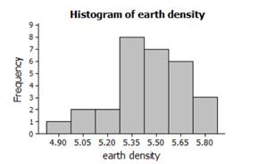
The measurements of the earth's density are roughly symmetric with a mean of 5.45 and vary from 4.88 to 5.85.
Shape: the distribution is roughly symmetric (part of the graph is a rough mirror image of the other part of the graph.)
The center is about 5.4479 (mean) or 5.46(median)
Spread is about 0.2209 (standard deviation)
Conclusion:
Therefore,
Shape: the distribution is roughly symmetric
The center 5.4479 (mean) or 5.46(median)
Spread: 0.2209 (standard deviation)
(b)
To find: the percent of observations that fall within one, two, and three standard deviations of the mean
(b)
Answer to Problem 64E
One standard deviations =
Two standard deviations = 96.55%
Three standard deviations = 100%
Explanation of Solution
The densities follow the
Conclusion:
Therefore,
One standard deviations =
Two standard deviations = 96.55%
Three standard deviations = 100%
(b)
To find: To construct: a Normal
(b)
Answer to Problem 64E
Explanation of Solution
Calculation:
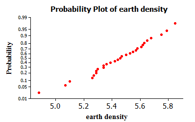
A Normal probability plot from Minitab is shown below:

The Normal probability plot is roughly linear, indicating that the densities are approximately Normal.
Conclusion:
Therefore, a Normal probability plot is plotted.
(b)
To explain: whether the data are approximately Normal
(b)
Answer to Problem 64E
the data are approximately Normal
Explanation of Solution
Calculation:
The graphical display in (A), check of the 68-95-99.7 rule in (B), and Normal probability plot in (C) indicate that these measurements are approximately Normal.
Conclusion:
Normal probability plot in (C) indicate that these measurements are approximately Normal.
Chapter 2 Solutions
The Practice of Statistics for AP - 4th Edition
Additional Math Textbook Solutions
College Algebra (7th Edition)
University Calculus: Early Transcendentals (4th Edition)
Calculus: Early Transcendentals (2nd Edition)
Basic Business Statistics, Student Value Edition
A First Course in Probability (10th Edition)
Algebra and Trigonometry (6th Edition)


- A biologist is investigating the effect of potential plant hormones by treating 20 stem segments. At the end of the observation period he computes the following length averages: Compound X = 1.18 Compound Y = 1.17 Based on these mean values he concludes that there are no treatment differences. 1) Are you satisfied with his conclusion? Why or why not? 2) If he asked you for help in analyzing these data, what statistical method would you suggest that he use to come to a meaningful conclusion about his data and why? 3) Are there any other questions you would ask him regarding his experiment, data collection, and analysis methods?arrow_forwardBusinessarrow_forwardWhat is the solution and answer to question?arrow_forward
- To: [Boss's Name] From: Nathaniel D Sain Date: 4/5/2025 Subject: Decision Analysis for Business Scenario Introduction to the Business Scenario Our delivery services business has been experiencing steady growth, leading to an increased demand for faster and more efficient deliveries. To meet this demand, we must decide on the best strategy to expand our fleet. The three possible alternatives under consideration are purchasing new delivery vehicles, leasing vehicles, or partnering with third-party drivers. The decision must account for various external factors, including fuel price fluctuations, demand stability, and competition growth, which we categorize as the states of nature. Each alternative presents unique advantages and challenges, and our goal is to select the most viable option using a structured decision-making approach. Alternatives and States of Nature The three alternatives for fleet expansion were chosen based on their cost implications, operational efficiency, and…arrow_forwardBusinessarrow_forwardWhy researchers are interested in describing measures of the center and measures of variation of a data set?arrow_forward
- WHAT IS THE SOLUTION?arrow_forwardThe following ordered data list shows the data speeds for cell phones used by a telephone company at an airport: A. Calculate the Measures of Central Tendency from the ungrouped data list. B. Group the data in an appropriate frequency table. C. Calculate the Measures of Central Tendency using the table in point B. 0.8 1.4 1.8 1.9 3.2 3.6 4.5 4.5 4.6 6.2 6.5 7.7 7.9 9.9 10.2 10.3 10.9 11.1 11.1 11.6 11.8 12.0 13.1 13.5 13.7 14.1 14.2 14.7 15.0 15.1 15.5 15.8 16.0 17.5 18.2 20.2 21.1 21.5 22.2 22.4 23.1 24.5 25.7 28.5 34.6 38.5 43.0 55.6 71.3 77.8arrow_forwardII Consider the following data matrix X: X1 X2 0.5 0.4 0.2 0.5 0.5 0.5 10.3 10 10.1 10.4 10.1 10.5 What will the resulting clusters be when using the k-Means method with k = 2. In your own words, explain why this result is indeed expected, i.e. why this clustering minimises the ESS map.arrow_forward
- why the answer is 3 and 10?arrow_forwardPS 9 Two films are shown on screen A and screen B at a cinema each evening. The numbers of people viewing the films on 12 consecutive evenings are shown in the back-to-back stem-and-leaf diagram. Screen A (12) Screen B (12) 8 037 34 7 6 4 0 534 74 1645678 92 71689 Key: 116|4 represents 61 viewers for A and 64 viewers for B A second stem-and-leaf diagram (with rows of the same width as the previous diagram) is drawn showing the total number of people viewing films at the cinema on each of these 12 evenings. Find the least and greatest possible number of rows that this second diagram could have. TIP On the evening when 30 people viewed films on screen A, there could have been as few as 37 or as many as 79 people viewing films on screen B.arrow_forwardQ.2.4 There are twelve (12) teams participating in a pub quiz. What is the probability of correctly predicting the top three teams at the end of the competition, in the correct order? Give your final answer as a fraction in its simplest form.arrow_forward
 MATLAB: An Introduction with ApplicationsStatisticsISBN:9781119256830Author:Amos GilatPublisher:John Wiley & Sons Inc
 Probability and Statistics for Engineering and th...StatisticsISBN:9781305251809Author:Jay L. DevorePublisher:Cengage Learning
 Statistics for The Behavioral Sciences (MindTap C...StatisticsISBN:9781305504912Author:Frederick J Gravetter, Larry B. WallnauPublisher:Cengage Learning
 Elementary Statistics: Picturing the World (7th E...StatisticsISBN:9780134683416Author:Ron Larson, Betsy FarberPublisher:PEARSON
 The Basic Practice of StatisticsStatisticsISBN:9781319042578Author:David S. Moore, William I. Notz, Michael A. FlignerPublisher:W. H. Freeman
 Introduction to the Practice of StatisticsStatisticsISBN:9781319013387Author:David S. Moore, George P. McCabe, Bruce A. CraigPublisher:W. H. Freeman