Concept explainers
Videos
(a)
To find: the proportion of observations from the standard
(a)
Answer to Problem 49E
The proportion of observations is 0.8587
Explanation of Solution
Given:
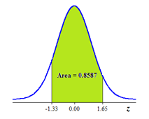
z is between −1.33 and 1.65
Calculation:
The below standard normal possibilities table is a table of areas under the standard normal curve. The table entry for each value z is the area under the curve to the left of z.
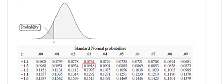
From the Standard Normal probabilities table, the area to the left of = = 1.65is 0.9505 and the area to the left of z = -1.33 is 0.0918.
The area between z = -1.33 and z =1.65is the area to the left of 1.65 minus the area to the left of -1.33.
Therefore, the area between z =-1.33 & z =1.65 is 0.9505 - 0.0918 =0.8587. The result is shown in the below graph.
Conclusion:
The proportion of observations is 0.8587
(b)
To find: the proportion of observations from the standard normal distribution
(b)
Answer to Problem 49E
The proportion of observations is0.2718.
Explanation of Solution
Given:
z is between 0.50 and 1.79
Calculation:
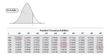
From the Standard Normal probabilities table, the area to the left of
The area between z = 0.50 and z =1.79is the area to the left of 1.79 minus the area to the left of 0.50.
Therefore, the area between z = 0.50 & z =1.79 is 0.9633 - 0.6915 =0.2718. The result is shown in the below graph
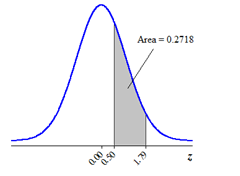
Conclusion:
Therefore, proportion of observations is 0.2718.
Chapter 2 Solutions
The Practice of Statistics for AP - 4th Edition
Additional Math Textbook Solutions
Introductory Statistics
Elementary Statistics (13th Edition)
College Algebra (7th Edition)
Intro Stats, Books a la Carte Edition (5th Edition)
Elementary Statistics: Picturing the World (7th Edition)


- Businessarrow_forwardWhat is the solution and answer to question?arrow_forwardTo: [Boss's Name] From: Nathaniel D Sain Date: 4/5/2025 Subject: Decision Analysis for Business Scenario Introduction to the Business Scenario Our delivery services business has been experiencing steady growth, leading to an increased demand for faster and more efficient deliveries. To meet this demand, we must decide on the best strategy to expand our fleet. The three possible alternatives under consideration are purchasing new delivery vehicles, leasing vehicles, or partnering with third-party drivers. The decision must account for various external factors, including fuel price fluctuations, demand stability, and competition growth, which we categorize as the states of nature. Each alternative presents unique advantages and challenges, and our goal is to select the most viable option using a structured decision-making approach. Alternatives and States of Nature The three alternatives for fleet expansion were chosen based on their cost implications, operational efficiency, and…arrow_forward
- The following ordered data list shows the data speeds for cell phones used by a telephone company at an airport: A. Calculate the Measures of Central Tendency from the ungrouped data list. B. Group the data in an appropriate frequency table. C. Calculate the Measures of Central Tendency using the table in point B. 0.8 1.4 1.8 1.9 3.2 3.6 4.5 4.5 4.6 6.2 6.5 7.7 7.9 9.9 10.2 10.3 10.9 11.1 11.1 11.6 11.8 12.0 13.1 13.5 13.7 14.1 14.2 14.7 15.0 15.1 15.5 15.8 16.0 17.5 18.2 20.2 21.1 21.5 22.2 22.4 23.1 24.5 25.7 28.5 34.6 38.5 43.0 55.6 71.3 77.8arrow_forwardII Consider the following data matrix X: X1 X2 0.5 0.4 0.2 0.5 0.5 0.5 10.3 10 10.1 10.4 10.1 10.5 What will the resulting clusters be when using the k-Means method with k = 2. In your own words, explain why this result is indeed expected, i.e. why this clustering minimises the ESS map.arrow_forwardwhy the answer is 3 and 10?arrow_forward
- PS 9 Two films are shown on screen A and screen B at a cinema each evening. The numbers of people viewing the films on 12 consecutive evenings are shown in the back-to-back stem-and-leaf diagram. Screen A (12) Screen B (12) 8 037 34 7 6 4 0 534 74 1645678 92 71689 Key: 116|4 represents 61 viewers for A and 64 viewers for B A second stem-and-leaf diagram (with rows of the same width as the previous diagram) is drawn showing the total number of people viewing films at the cinema on each of these 12 evenings. Find the least and greatest possible number of rows that this second diagram could have. TIP On the evening when 30 people viewed films on screen A, there could have been as few as 37 or as many as 79 people viewing films on screen B.arrow_forwardQ.2.4 There are twelve (12) teams participating in a pub quiz. What is the probability of correctly predicting the top three teams at the end of the competition, in the correct order? Give your final answer as a fraction in its simplest form.arrow_forwardThe table below indicates the number of years of experience of a sample of employees who work on a particular production line and the corresponding number of units of a good that each employee produced last month. Years of Experience (x) Number of Goods (y) 11 63 5 57 1 48 4 54 5 45 3 51 Q.1.1 By completing the table below and then applying the relevant formulae, determine the line of best fit for this bivariate data set. Do NOT change the units for the variables. X y X2 xy Ex= Ey= EX2 EXY= Q.1.2 Estimate the number of units of the good that would have been produced last month by an employee with 8 years of experience. Q.1.3 Using your calculator, determine the coefficient of correlation for the data set. Interpret your answer. Q.1.4 Compute the coefficient of determination for the data set. Interpret your answer.arrow_forward
 MATLAB: An Introduction with ApplicationsStatisticsISBN:9781119256830Author:Amos GilatPublisher:John Wiley & Sons Inc
 Probability and Statistics for Engineering and th...StatisticsISBN:9781305251809Author:Jay L. DevorePublisher:Cengage Learning
 Statistics for The Behavioral Sciences (MindTap C...StatisticsISBN:9781305504912Author:Frederick J Gravetter, Larry B. WallnauPublisher:Cengage Learning
 Elementary Statistics: Picturing the World (7th E...StatisticsISBN:9780134683416Author:Ron Larson, Betsy FarberPublisher:PEARSON
 The Basic Practice of StatisticsStatisticsISBN:9781319042578Author:David S. Moore, William I. Notz, Michael A. FlignerPublisher:W. H. Freeman
 Introduction to the Practice of StatisticsStatisticsISBN:9781319013387Author:David S. Moore, George P. McCabe, Bruce A. CraigPublisher:W. H. Freeman