Statistics Through Applications
2nd Edition
ISBN: 9781429219747
Author: Daren S. Starnes, David Moore, Dan Yates
Publisher: Macmillan Higher Education
expand_more
expand_more
format_list_bulleted
Videos
Question
Chapter 2.2, Problem 2.43E
To determine
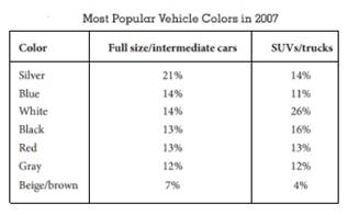
To construct: the graph which compares the colours distribution for full size/intermediate cars and SUV/trucks.
Expert Solution & Answer
Explanation of Solution
Given:
Graph:
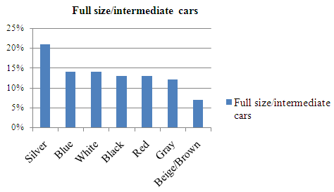
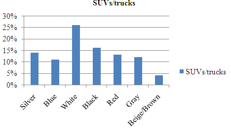
By seeing both the graphs which are similar in this way that the same categories and beige/brown is the least popular in both the graphs but there is difference in the full size/intermediate cars category the silver cars are almost popular while in the SUV/trucks category the white cars are the most popular
Chapter 2 Solutions
Statistics Through Applications
Ch. 2.1 - Prob. 2.1ECh. 2.1 - Prob. 2.2ECh. 2.1 - Prob. 2.3ECh. 2.1 - Prob. 2.4ECh. 2.1 - Prob. 2.5ECh. 2.1 - Prob. 2.6ECh. 2.1 - Prob. 2.7ECh. 2.1 - Prob. 2.8ECh. 2.1 - Prob. 2.9ECh. 2.1 - Prob. 2.10E
Ch. 2.1 - Prob. 2.11ECh. 2.1 - Prob. 2.12ECh. 2.1 - Prob. 2.13ECh. 2.1 - Prob. 2.14ECh. 2.1 - Prob. 2.15ECh. 2.1 - Prob. 2.16ECh. 2.1 - Prob. 2.17ECh. 2.1 - Prob. 2.19ECh. 2.1 - Prob. 2.20ECh. 2.1 - Prob. 2.21ECh. 2.1 - Prob. 2.23ECh. 2.1 - Prob. 2.24ECh. 2.1 - Prob. 2.25ECh. 2.1 - Prob. 2.26ECh. 2.2 - Prob. 2.27ECh. 2.2 - Prob. 2.28ECh. 2.2 - Prob. 2.29ECh. 2.2 - Prob. 2.30ECh. 2.2 - Prob. 2.31ECh. 2.2 - Prob. 2.32ECh. 2.2 - Prob. 2.33ECh. 2.2 - Prob. 2.34ECh. 2.2 - Prob. 2.35ECh. 2.2 - Prob. 2.36ECh. 2.2 - Prob. 2.37ECh. 2.2 - Prob. 2.38ECh. 2.2 - Prob. 2.39ECh. 2.2 - Prob. 2.40ECh. 2.2 - Prob. 2.41ECh. 2.2 - Prob. 2.42ECh. 2.2 - Prob. 2.43ECh. 2.2 - Prob. 2.44ECh. 2.2 - Prob. 2.45ECh. 2.2 - Prob. 2.46ECh. 2.2 - Prob. 2.47ECh. 2.2 - Prob. 2.48ECh. 2.2 - Prob. 2.49ECh. 2.2 - Prob. 2.50ECh. 2.2 - Prob. 2.51ECh. 2.2 - Prob. 2.52ECh. 2.3 - Prob. 2.53ECh. 2.3 - Prob. 2.54ECh. 2.3 - Prob. 2.55ECh. 2.3 - Prob. 2.56ECh. 2.3 - Prob. 2.57ECh. 2.3 - Prob. 2.58ECh. 2.3 - Prob. 2.59ECh. 2.3 - Prob. 2.60ECh. 2.3 - Prob. 2.61ECh. 2.3 - Prob. 2.62ECh. 2.3 - Prob. 2.63ECh. 2.3 - Prob. 2.64ECh. 2.3 - Prob. 2.65ECh. 2 - Prob. 2.67RECh. 2 - Prob. 2.68RECh. 2 - Prob. 2.69RECh. 2 - Prob. 2.70RECh. 2 - Prob. 2.71RECh. 2 - Prob. 2.72RECh. 2 - Prob. 2.73RECh. 2 - Prob. 2.74RECh. 2 - Prob. 2.75RECh. 2 - Prob. 2.76RE
Additional Math Textbook Solutions
Find more solutions based on key concepts
Consider an experiment that consists of determining the type of job-either blue collar or white collar-and the ...
A First Course in Probability (10th Edition)
The solution of the given equation
Pre-Algebra Student Edition
For a population containing N=902 individual, what code number would you assign for a. the first person on the ...
Basic Business Statistics, Student Value Edition
Mathematical Connections Explain why 25 cents is one-fourth of a dollar, yet 15 minutes is one-fourth of an hou...
A Problem Solving Approach To Mathematics For Elementary School Teachers (13th Edition)
Knowledge Booster


Learn more about
Need a deep-dive on the concept behind this application? Look no further. Learn more about this topic, statistics and related others by exploring similar questions and additional content below.Similar questions
- Problem 3. Pricing a multi-stock option the Margrabe formula The purpose of this problem is to price a swap option in a 2-stock model, similarly as what we did in the example in the lectures. We consider a two-dimensional Brownian motion given by W₁ = (W(¹), W(2)) on a probability space (Q, F,P). Two stock prices are modeled by the following equations: dX = dY₁ = X₁ (rdt+ rdt+0₁dW!) (²)), Y₁ (rdt+dW+0zdW!"), with Xo xo and Yo =yo. This corresponds to the multi-stock model studied in class, but with notation (X+, Y₁) instead of (S(1), S(2)). Given the model above, the measure P is already the risk-neutral measure (Both stocks have rate of return r). We write σ = 0₁+0%. We consider a swap option, which gives you the right, at time T, to exchange one share of X for one share of Y. That is, the option has payoff F=(Yr-XT). (a) We first assume that r = 0 (for questions (a)-(f)). Write an explicit expression for the process Xt. Reminder before proceeding to question (b): Girsanov's theorem…arrow_forwardProblem 1. Multi-stock model We consider a 2-stock model similar to the one studied in class. Namely, we consider = S(1) S(2) = S(¹) exp (σ1B(1) + (M1 - 0/1 ) S(²) exp (02B(2) + (H₂- M2 where (B(¹) ) +20 and (B(2) ) +≥o are two Brownian motions, with t≥0 Cov (B(¹), B(2)) = p min{t, s}. " The purpose of this problem is to prove that there indeed exists a 2-dimensional Brownian motion (W+)+20 (W(1), W(2))+20 such that = S(1) S(2) = = S(¹) exp (011W(¹) + (μ₁ - 01/1) t) 롱) S(²) exp (021W (1) + 022W(2) + (112 - 03/01/12) t). where σ11, 21, 22 are constants to be determined (as functions of σ1, σ2, p). Hint: The constants will follow the formulas developed in the lectures. (a) To show existence of (Ŵ+), first write the expression for both W. (¹) and W (2) functions of (B(1), B(²)). as (b) Using the formulas obtained in (a), show that the process (WA) is actually a 2- dimensional standard Brownian motion (i.e. show that each component is normal, with mean 0, variance t, and that their…arrow_forwardThe scores of 8 students on the midterm exam and final exam were as follows. Student Midterm Final Anderson 98 89 Bailey 88 74 Cruz 87 97 DeSana 85 79 Erickson 85 94 Francis 83 71 Gray 74 98 Harris 70 91 Find the value of the (Spearman's) rank correlation coefficient test statistic that would be used to test the claim of no correlation between midterm score and final exam score. Round your answer to 3 places after the decimal point, if necessary. Test statistic: rs =arrow_forward
- Business discussarrow_forwardBusiness discussarrow_forwardI just need to know why this is wrong below: What is the test statistic W? W=5 (incorrect) and What is the p-value of this test? (p-value < 0.001-- incorrect) Use the Wilcoxon signed rank test to test the hypothesis that the median number of pages in the statistics books in the library from which the sample was taken is 400. A sample of 12 statistics books have the following numbers of pages pages 127 217 486 132 397 297 396 327 292 256 358 272 What is the sum of the negative ranks (W-)? 75 What is the sum of the positive ranks (W+)? 5What type of test is this? two tailedWhat is the test statistic W? 5 These are the critical values for a 1-tailed Wilcoxon Signed Rank test for n=12 Alpha Level 0.001 0.005 0.01 0.025 0.05 0.1 0.2 Critical Value 75 70 68 64 60 56 50 What is the p-value for this test? p-value < 0.001arrow_forward
- ons 12. A sociologist hypothesizes that the crime rate is higher in areas with higher poverty rate and lower median income. She col- lects data on the crime rate (crimes per 100,000 residents), the poverty rate (in %), and the median income (in $1,000s) from 41 New England cities. A portion of the regression results is shown in the following table. Standard Coefficients error t stat p-value Intercept -301.62 549.71 -0.55 0.5864 Poverty 53.16 14.22 3.74 0.0006 Income 4.95 8.26 0.60 0.5526 a. b. Are the signs as expected on the slope coefficients? Predict the crime rate in an area with a poverty rate of 20% and a median income of $50,000. 3. Using data from 50 workarrow_forward2. The owner of several used-car dealerships believes that the selling price of a used car can best be predicted using the car's age. He uses data on the recent selling price (in $) and age of 20 used sedans to estimate Price = Po + B₁Age + ε. A portion of the regression results is shown in the accompanying table. Standard Coefficients Intercept 21187.94 Error 733.42 t Stat p-value 28.89 1.56E-16 Age -1208.25 128.95 -9.37 2.41E-08 a. What is the estimate for B₁? Interpret this value. b. What is the sample regression equation? C. Predict the selling price of a 5-year-old sedan.arrow_forwardian income of $50,000. erty rate of 13. Using data from 50 workers, a researcher estimates Wage = Bo+B,Education + B₂Experience + B3Age+e, where Wage is the hourly wage rate and Education, Experience, and Age are the years of higher education, the years of experience, and the age of the worker, respectively. A portion of the regression results is shown in the following table. ni ogolloo bash 1 Standard Coefficients error t stat p-value Intercept 7.87 4.09 1.93 0.0603 Education 1.44 0.34 4.24 0.0001 Experience 0.45 0.14 3.16 0.0028 Age -0.01 0.08 -0.14 0.8920 a. Interpret the estimated coefficients for Education and Experience. b. Predict the hourly wage rate for a 30-year-old worker with four years of higher education and three years of experience.arrow_forward
- 1. If a firm spends more on advertising, is it likely to increase sales? Data on annual sales (in $100,000s) and advertising expenditures (in $10,000s) were collected for 20 firms in order to estimate the model Sales = Po + B₁Advertising + ε. A portion of the regression results is shown in the accompanying table. Intercept Advertising Standard Coefficients Error t Stat p-value -7.42 1.46 -5.09 7.66E-05 0.42 0.05 8.70 7.26E-08 a. Interpret the estimated slope coefficient. b. What is the sample regression equation? C. Predict the sales for a firm that spends $500,000 annually on advertising.arrow_forwardCan you help me solve problem 38 with steps im stuck.arrow_forwardHow do the samples hold up to the efficiency test? What percentages of the samples pass or fail the test? What would be the likelihood of having the following specific number of efficiency test failures in the next 300 processors tested? 1 failures, 5 failures, 10 failures and 20 failures.arrow_forward
arrow_back_ios
SEE MORE QUESTIONS
arrow_forward_ios
Recommended textbooks for you
 MATLAB: An Introduction with ApplicationsStatisticsISBN:9781119256830Author:Amos GilatPublisher:John Wiley & Sons Inc
 Probability and Statistics for Engineering and th...StatisticsISBN:9781305251809Author:Jay L. DevorePublisher:Cengage Learning
 Statistics for The Behavioral Sciences (MindTap C...StatisticsISBN:9781305504912Author:Frederick J Gravetter, Larry B. WallnauPublisher:Cengage Learning
 Elementary Statistics: Picturing the World (7th E...StatisticsISBN:9780134683416Author:Ron Larson, Betsy FarberPublisher:PEARSON
 The Basic Practice of StatisticsStatisticsISBN:9781319042578Author:David S. Moore, William I. Notz, Michael A. FlignerPublisher:W. H. Freeman
 Introduction to the Practice of StatisticsStatisticsISBN:9781319013387Author:David S. Moore, George P. McCabe, Bruce A. CraigPublisher:W. H. Freeman
MATLAB: An Introduction with Applications
Statistics
ISBN:9781119256830
Author:Amos Gilat
Publisher:John Wiley & Sons Inc
Probability and Statistics for Engineering and th...
Statistics
ISBN:9781305251809
Author:Jay L. Devore
Publisher:Cengage Learning
Statistics for The Behavioral Sciences (MindTap C...
Statistics
ISBN:9781305504912
Author:Frederick J Gravetter, Larry B. Wallnau
Publisher:Cengage Learning
Elementary Statistics: Picturing the World (7th E...
Statistics
ISBN:9780134683416
Author:Ron Larson, Betsy Farber
Publisher:PEARSON
The Basic Practice of Statistics
Statistics
ISBN:9781319042578
Author:David S. Moore, William I. Notz, Michael A. Fligner
Publisher:W. H. Freeman
Introduction to the Practice of Statistics
Statistics
ISBN:9781319013387
Author:David S. Moore, George P. McCabe, Bruce A. Craig
Publisher:W. H. Freeman
How to make Frequency Distribution Table / Tally Marks and Frequency Distribution Table; Author: Reenu Math;https://www.youtube.com/watch?v=i_A6RiE8tLE;License: Standard YouTube License, CC-BY
Frequency distribution table in statistics; Author: Math and Science;https://www.youtube.com/watch?v=T7KYO76DoOE;License: Standard YouTube License, CC-BY
Frequency Distribution Table for Grouped/Continuous data | Math Dot Com; Author: Maths dotcom;https://www.youtube.com/watch?v=ErnccbXQOPY;License: Standard Youtube License