Concept explainers
Videos
a.
Construct a frequency distribution for the data.
a.
Answer to Problem 21E
The frequency distribution is obtained as shown below:
| Revenue | Frequency |
| 0-49 | 6 |
| 50-99 | 29 |
| 100-149 | 11 |
| 150-199 | 0 |
| 200-249 | 1 |
| 250-299 | 1 |
| 300-349 | 0 |
| 350-399 | 0 |
| 400-449 | 2 |
| Total | 50 |
Explanation of Solution
Calculation:
The data represent the list of 50 Country A’s largest corporations with annual revenue expressed in billions of dollars and the frequency distribution is constructed using the classes 0-49, 50-99,100-149, and so on.
Frequency:
The frequencies are calculated using the tally mark and the
- Based on the given information, the class intervals are 0-49, 50-99, 100-149, …,400-449.
- Make a tally mark for each value in the corresponding revenue class and continue for all the values in the data.
- The number of tally marks in each class represents the frequency, f, of that class.
Similarly, the frequency of the remaining classes for the revenue is given below:
| Revenue | Tally | Frequency |
| 0-49 | 6 | |
| 50-99 | 29 | |
| 100-149 | 11 | |
| 150-199 | 0 | |
| 200-249 | 1 | |
| 250-299 | 1 | |
| 300-349 | 0 | |
| 350-399 | 0 | |
| 400-449 | 2 | |
| Total | 50 |
b.
Construct a relative frequency distribution for the data.
b.
Answer to Problem 21E
The relative frequency distribution is tabulated below:
| Revenue | Frequency | Relative frequency |
| 0-49 | 6 | 0.12 |
| 50-99 | 29 | 0.58 |
| 100-149 | 11 | 0.22 |
| 150-199 | 0 | 0.00 |
| 200-249 | 1 | 0.02 |
| 250-299 | 1 | 0.02 |
| 300-349 | 0 | 0.00 |
| 350-399 | 0 | 0.00 |
| 400-449 | 2 | 0.04 |
| Total | 50 | 1.00 |
Explanation of Solution
Calculation:
Relative frequency:
The general formula for the relative frequency is as follows:
For the revenue class (0-49), substitute frequency as “6” and total frequency as “50”.
Similarly, the relative frequencies for the remaining revenue classes are obtained below:
| Revenue | Frequency | Relative frequency |
| 0-49 | 6 | 0.12 |
| 50-99 | 29 | 0.58 |
| 100-149 | 11 | 0.22 |
| 150-199 | 0 | 0.00 |
| 200-249 | 1 | 0.02 |
| 250-299 | 1 | 0.02 |
| 300-349 | 0 | 0.00 |
| 350-399 | 0 | 0.00 |
| 400-449 | 2 | 0.04 |
| Total | 50 | 1.00 |
c.
Construct a cumulative frequency distribution for the data.
c.
Answer to Problem 21E
The cumulative frequency distribution is as follows:
| Revenue | Frequency | Cumulative frequency |
| 0-49 | 6 | 6 |
| 50-99 | 29 | 35 |
| 100-149 | 11 | 46 |
| 150-199 | 0 | 46 |
| 200-249 | 1 | 47 |
| 250-299 | 1 | 48 |
| 300-349 | 0 | 48 |
| 350-399 | 0 | 48 |
| 400-449 | 2 | 50 |
Explanation of Solution
Calculation:
Cumulative frequency:
Cumulative frequency of a particular class is the sum of all frequencies up to a class. The last class’s cumulative frequency is equal to the
Thus, the cumulative frequency for each class is tabulated below:
The relative frequencies for the five types of classes are obtained below:
| Revenue | Frequency | Cumulative frequency |
| 0-49 | 6 | 6 |
| 50-99 | 29 | |
| 100-149 | 11 | |
| 150-199 | 0 | |
| 200-249 | 1 | |
| 250-299 | 1 | |
| 300-349 | 0 | |
| 350-399 | 0 | |
| 400-449 | 2 |
d.
Construct a cumulative relative frequency distribution for the data.
d.
Answer to Problem 21E
The cumulative relative frequency distribution is given below:
| Revenue | Cumulative relative frequency |
| 0-49 | 0.12 |
| 50-99 | 0.70 |
| 100-149 | 0.92 |
| 150-199 | 0.92 |
| 200-249 | 0.94 |
| 250-299 | 0.96 |
| 300-349 | 0.96 |
| 350-399 | 0.96 |
| 400-449 | 1.00 |
Explanation of Solution
Calculation:
Cumulative relative frequency of a particular class is the sum of all relative frequencies up to a class. The last class’s cumulative relative frequency is equal to the approximate value 1.00.
The relative frequencies for the revenue classes from part (b) is given below:
| Revenue | Frequency | Relative frequency |
| 0-49 | 6 | 0.12 |
| 50-99 | 29 | 0.58 |
| 100-149 | 11 | 0.22 |
| 150-199 | 0 | 0.00 |
| 200-249 | 1 | 0.02 |
| 250-299 | 1 | 0.02 |
| 300-349 | 0 | 0.00 |
| 350-399 | 0 | 0.00 |
| 400-449 | 2 | 0.04 |
| Total | 50 | 1.00 |
Thus, the cumulative relative frequencies for the revenue classes are obtained below:
| Revenue | Relative frequency | Cumulative relative frequency |
| 0-49 | 0.12 | 0.12 |
| 50-99 | 0.58 | |
| 100-149 | 0.22 | |
| 150-199 | 0.00 | |
| 200-249 | 0.02 | |
| 250-299 | 0.02 | |
| 300-349 | 0.00 | |
| 350-399 | 0.00 | |
| 400-449 | 0.04 |
e.
Explain about the annual revenue of the largest corporations in Country A using the distributions.
e.
Explanation of Solution
From the given data set and obtained distributions, it is observed that the frequency for the revenues in the range of 50 billion dollars to 149 billion dollars is obtained by the majority of 40 corporations over 50 largest corporations.
Further, the revenue over $200 billion is obtained by only 4 corporations and the revenue over 400 billion dollars is obtained by only 2 corporations.
Moreover, 70 percent of the corporations have revenues under 100 billion dollars. Only 30 percent of corporations have revenues over 100 billion dollars.
f.
Construct the histogram and comment on the shape of the distribution.
f.
Answer to Problem 21E
- The histogram of the data is given below:
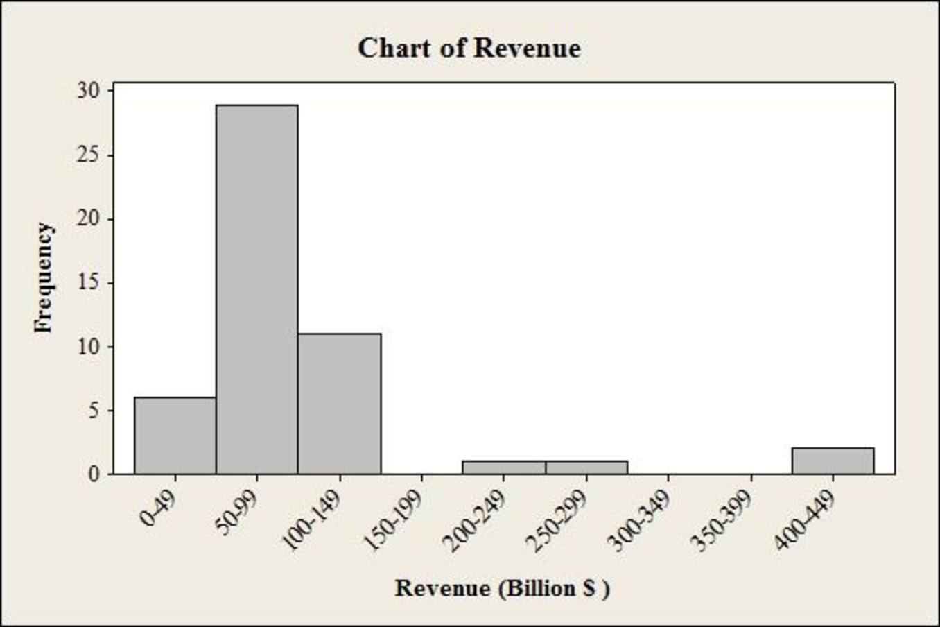
The histogram is skewed to the right.
Explanation of Solution
Calculation:
Software procedure:
Step-by-step procedure to draw the frequency histogram chart using MINITAB software:
- Choose Graph > Histogram.
- Choose Simple, and then click OK.
- In Graph variables, enter the Revenue column of data.
- In scale on y-axis, make click on frequency.
- Click on ok.
Skewness:
The data are said to be skewed if there is a lack of symmetry and the values fall on one side, that is, either left or right of the distribution.
Right skewed:
If the tail on the distribution is elongated toward the right and it attains its peak rapidly than its horizontal axis, then it is a right-skewed distribution. It is also called positively skewed.
The distribution of revenue in the histogram has elongated tail toward the right side. There are four corporations in the range of 200 billion dollars to 449 billion dollars.
Therefore, the distribution of the histogram with revenue is skewed to the right.
g.
Find the largest corporation in Country A and find its annual revenue.
g.
Answer to Problem 21E
Exxon-Mobil is the largest corporation in Country A and its annual revenue is 443 billion dollars.
Explanation of Solution
From the data set of 50 largest corporations, it is observed that the largest corporation in Country A is Exxon-Mobil and its annual revenue is 443 billion dollars.
The second largest corporation in Country A is Walmart and its annual revenue is 406 billion dollars.
Moreover, the possibility of corporation that has annual revenues less than 150 billion dollars is approximately 92 percent, and the remaining other corporations have annual revenues less than 300 billion dollars.
Want to see more full solutions like this?
Chapter 2 Solutions
Essentials of Statistics for Business and Economics (with XLSTAT Printed Access Card)


- Questions An insurance company's cumulative incurred claims for the last 5 accident years are given in the following table: Development Year Accident Year 0 2018 1 2 3 4 245 267 274 289 292 2019 255 276 288 294 2020 265 283 292 2021 263 278 2022 271 It can be assumed that claims are fully run off after 4 years. The premiums received for each year are: Accident Year Premium 2018 306 2019 312 2020 318 2021 326 2022 330 You do not need to make any allowance for inflation. 1. (a) Calculate the reserve at the end of 2022 using the basic chain ladder method. (b) Calculate the reserve at the end of 2022 using the Bornhuetter-Ferguson method. 2. Comment on the differences in the reserves produced by the methods in Part 1.arrow_forwardTo help consumers in purchasing a laptop computer, Consumer Reports calculates an overall test score for each computer tested based upon rating factors such as ergonomics, portability, performance, display, and battery life. Higher overall scores indicate better test results. The following data show the average retail price and the overall score for ten 13-inch models (Consumer Reports website, October 25, 2012). Brand & Model Price ($) Overall Score Samsung Ultrabook NP900X3C-A01US 1250 83 Apple MacBook Air MC965LL/A 1300 83 Apple MacBook Air MD231LL/A 1200 82 HP ENVY 13-2050nr Spectre XT 950 79 Sony VAIO SVS13112FXB 800 77 Acer Aspire S5-391-9880 Ultrabook 1200 74 Apple MacBook Pro MD101LL/A 1200 74 Apple MacBook Pro MD313LL/A 1000 73 Dell Inspiron I13Z-6591SLV 700 67 Samsung NP535U3C-A01US 600 63 a. Select a scatter diagram with price as the independent variable. b. What does the scatter diagram developed in part (a) indicate about the relationship…arrow_forwardTo the Internal Revenue Service, the reasonableness of total itemized deductions depends on the taxpayer’s adjusted gross income. Large deductions, which include charity and medical deductions, are more reasonable for taxpayers with large adjusted gross incomes. If a taxpayer claims larger than average itemized deductions for a given level of income, the chances of an IRS audit are increased. Data (in thousands of dollars) on adjusted gross income and the average or reasonable amount of itemized deductions follow. Adjusted Gross Income ($1000s) Reasonable Amount ofItemized Deductions ($1000s) 22 9.6 27 9.6 32 10.1 48 11.1 65 13.5 85 17.7 120 25.5 Compute b1 and b0 (to 4 decimals).b1 b0 Complete the estimated regression equation (to 2 decimals). = + x Predict a reasonable level of total itemized deductions for a taxpayer with an adjusted gross income of $52.5 thousand (to 2 decimals). thousand dollarsWhat is the value, in dollars, of…arrow_forward
- K The mean height of women in a country (ages 20-29) is 63.7 inches. A random sample of 65 women in this age group is selected. What is the probability that the mean height for the sample is greater than 64 inches? Assume σ = 2.68. The probability that the mean height for the sample is greater than 64 inches is (Round to four decimal places as needed.)arrow_forwardIn a survey of a group of men, the heights in the 20-29 age group were normally distributed, with a mean of 69.6 inches and a standard deviation of 4.0 inches. A study participant is randomly selected. Complete parts (a) through (d) below. (a) Find the probability that a study participant has a height that is less than 68 inches. The probability that the study participant selected at random is less than 68 inches tall is 0.4. (Round to four decimal places as needed.) 20 2arrow_forwardPEER REPLY 1: Choose a classmate's Main Post and review their decision making process. 1. Choose a risk level for each of the states of nature (assign a probability value to each). 2. Explain why each risk level is chosen. 3. Which alternative do you believe would be the best based on the maximum EMV? 4. Do you feel determining the expected value with perfect information (EVWPI) is worthwhile in this situation? Why or why not?arrow_forward
- Questions An insurance company's cumulative incurred claims for the last 5 accident years are given in the following table: Development Year Accident Year 0 2018 1 2 3 4 245 267 274 289 292 2019 255 276 288 294 2020 265 283 292 2021 263 278 2022 271 It can be assumed that claims are fully run off after 4 years. The premiums received for each year are: Accident Year Premium 2018 306 2019 312 2020 318 2021 326 2022 330 You do not need to make any allowance for inflation. 1. (a) Calculate the reserve at the end of 2022 using the basic chain ladder method. (b) Calculate the reserve at the end of 2022 using the Bornhuetter-Ferguson method. 2. Comment on the differences in the reserves produced by the methods in Part 1.arrow_forwardYou are provided with data that includes all 50 states of the United States. Your task is to draw a sample of: o 20 States using Random Sampling (2 points: 1 for random number generation; 1 for random sample) o 10 States using Systematic Sampling (4 points: 1 for random numbers generation; 1 for random sample different from the previous answer; 1 for correct K value calculation table; 1 for correct sample drawn by using systematic sampling) (For systematic sampling, do not use the original data directly. Instead, first randomize the data, and then use the randomized dataset to draw your sample. Furthermore, do not use the random list previously generated, instead, generate a new random sample for this part. For more details, please see the snapshot provided at the end.) Upload a Microsoft Excel file with two separate sheets. One sheet provides random sampling while the other provides systematic sampling. Excel snapshots that can help you in organizing columns are provided on the next…arrow_forwardThe population mean and standard deviation are given below. Find the required probability and determine whether the given sample mean would be considered unusual. For a sample of n = 65, find the probability of a sample mean being greater than 225 if μ = 224 and σ = 3.5. For a sample of n = 65, the probability of a sample mean being greater than 225 if μ=224 and σ = 3.5 is 0.0102 (Round to four decimal places as needed.)arrow_forward
- ***Please do not just simply copy and paste the other solution for this problem posted on bartleby as that solution does not have all of the parts completed for this problem. Please answer this I will leave a like on the problem. The data needed to answer this question is given in the following link (file is on view only so if you would like to make a copy to make it easier for yourself feel free to do so) https://docs.google.com/spreadsheets/d/1aV5rsxdNjHnkeTkm5VqHzBXZgW-Ptbs3vqwk0SYiQPo/edit?usp=sharingarrow_forwardThe data needed to answer this question is given in the following link (file is on view only so if you would like to make a copy to make it easier for yourself feel free to do so) https://docs.google.com/spreadsheets/d/1aV5rsxdNjHnkeTkm5VqHzBXZgW-Ptbs3vqwk0SYiQPo/edit?usp=sharingarrow_forwardThe following relates to Problems 4 and 5. Christchurch, New Zealand experienced a major earthquake on February 22, 2011. It destroyed 100,000 homes. Data were collected on a sample of 300 damaged homes. These data are saved in the file called CIEG315 Homework 4 data.xlsx, which is available on Canvas under Files. A subset of the data is shown in the accompanying table. Two of the variables are qualitative in nature: Wall construction and roof construction. Two of the variables are quantitative: (1) Peak ground acceleration (PGA), a measure of the intensity of ground shaking that the home experienced in the earthquake (in units of acceleration of gravity, g); (2) Damage, which indicates the amount of damage experienced in the earthquake in New Zealand dollars; and (3) Building value, the pre-earthquake value of the home in New Zealand dollars. PGA (g) Damage (NZ$) Building Value (NZ$) Wall Construction Roof Construction Property ID 1 0.645 2 0.101 141,416 2,826 253,000 B 305,000 B T 3…arrow_forward
 Holt Mcdougal Larson Pre-algebra: Student Edition...AlgebraISBN:9780547587776Author:HOLT MCDOUGALPublisher:HOLT MCDOUGAL
 Glencoe Algebra 1, Student Edition, 9780079039897...AlgebraISBN:9780079039897Author:CarterPublisher:McGraw Hill
 Big Ideas Math A Bridge To Success Algebra 1: Stu...AlgebraISBN:9781680331141Author:HOUGHTON MIFFLIN HARCOURTPublisher:Houghton Mifflin Harcourt