
Videos
Protein Grams in Fast Food The amount of protein (in grams) for a variety of fast-food sandwiches is reported here. Construct a frequency distribution, using 6 classes. Draw a histogram, a frequency
To Sketch: A histogram, frequency polygon and ogive using relative frequency and describe the shape of the histogram for the given data.
Answer to Problem 18E
The sketches of all three graphs are as follows:
The shape of the histogram is right skewed.
Explanation of Solution
Given Info:
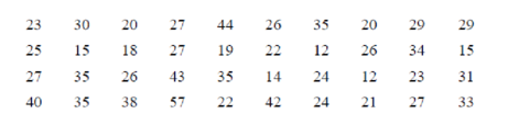
The amount of protein (in grams) for a variety of fast-food sandwiches is reported here
| 23 | 30 | 20 | 27 | 44 | 26 | 35 | 20 | 29 | 29 |
| 25 | 15 | 18 | 27 | 19 | 22 | 12 | 26 | 34 | 15 |
| 27 | 35 | 26 | 43 | 35 | 14 | 24 | 12 | 23 | 31 |
| 40 | 35 | 38 | 57 | 22 | 42 | 24 | 21 | 27 | 33 |
Calculation:
The class boundaries for any class are given by:
The grouped frequency distribution is as follows:
| Class limit | Class boundaries |  Tally Tally |
Frequency |
| 12-19 | 11.5-19.5 |  |
7 |
| 20-27 | 19.5-27.5 |  |
17 |
| 28-35 | 27.5-35.5 | 10 | |
| 36-43 | 35.5-43.5 |
|
4 |
| 44-51 | 43.5-51.5 |
|
1 |
| 52-59 | 51.5-59.5 |
|
1 |
Class midpoint:
The midpoint of class boundaries is obtained by adding lower and upper limit and dividing by 2.
For the first class,
Thus, the midpoint for the first class is 22.
Similarly, the midpoint for other classes was obtained.
Relative frequency distribution:
The relative frequency is the ration of a class frequency to the total frequency. Cumulative relative frequency can also defined as the sum of all previous frequencies up to the current point.
| Class boundaries | Frequency | Mid point |
Relative frequency |
Cumulative relative frequency |
| 11.5-19.5 | 7 | 15.5 | 0.175 | 0.175 |
| 19.5-27.5 | 17 | 23.5 | 0.425 | 0.6 |
| 27.5-35.5 | 10 | 31.5 | 0.25 | 0.85 |
| 35.5-43.5 | 4 | 39.5 | 0.1 | 0.95 |
| 43.5-51.5 | 1 | 47.5 | 0.025 | 0.975 |
| 51.5-59.5 | 1 | 55.5 | 0.025 | 1 |
| Total | 40 |
The histogram is a graph that displays the data by using contiguous vertical bars of various heights to represent the frequencies of the classes.
| Upper limit | Relative frequency |
| 19.5 | 0.175 |
| 27.5 | 0.425 |
| 35.5 | 0.25 |
| 43.5 | 0.1 |
| 51.5 | 0.025 |
| 59.5 | 0.025 |
Histogram:
Software procedure:
Step by step procedure for constructing histogram using Excel is given below:
- Press [Ctrl]-N for a new workbook.
- Enter the data in column A, one number per cell.
- Enter the upper boundaries into column B.
- From the toolbar, select the Data tab, then select Data Analysis.
- In Data Analysis, select Histogram and click [OK].
- In the Histogram dialog box, select relative column in the Input Range box and select upper limit column in the Bin Range box.
- Select New Worksheet Ply and Chart Output. Click [OK].
Output obtained from Excel is given below:
Shape of the distribution:
Symmetric:
A distribution is said to be symmetric if the left side of histogram is the mirror image of the right side of histogram.
Skewed right:
If the right side of the distribution extends far away than the left side of histogram, it is said to be skewed right.
Skewed left:
If the left side of the distribution extends far away than the right side of histogram, it is said to be skewed left.
Here, the histogram extends far away than the left side of histogram, it is said to be skewed right.
Hence, the distribution for the amount of protein (in grams) for a variety of fast-food sandwiches is skewed right.
Frequency polygons:
Step by step procedure for constructing frequency polygon using Excel is given below:
- Press [CTRL]-N for a new notebook.
- Enter the midpoints of the data into column A and the frequencies into column B including labels.
- Press and hold the left mouse button, and drag over the Frequencies (including the label) from column B.
- Select the Insert tab from the toolbar and the Line Chart option.
- Select the 2-D line chart type.
Output obtained from Excel is given below:

Frequency ogive:
Step by step procedure for constructing frequency ogive using Excel is given below:
- To create an ogive, use the upper class boundaries (horizontal axis) and cumulative frequencies (vertical axis) from the frequency distribution.
- Type the upper class boundaries (including a class with frequency 0 before the lowest class to anchor the graph to the horizontal axis) and
- Corresponding cumulative frequencies into adjacent columns of an Excel worksheet.
- Press and hold the left mouse button, and drag over the Cumulative Frequencies from column B.
- Select Line Chart, then the 2-D Line option.
Output obtained from Excel is given below:

The points plotted are the upper class limit and the corresponding cumulative relative frequency.
Want to see more full solutions like this?
Chapter 2 Solutions
Connect Plus Statistics Hosted by ALEKS Access Card 52 Weeks for Elementary Statistics: A Step-By-St


- Suppose a random sample of 459 married couples found that 307 had two or more personality preferences in common. In another random sample of 471 married couples, it was found that only 31 had no preferences in common. Let p1 be the population proportion of all married couples who have two or more personality preferences in common. Let p2 be the population proportion of all married couples who have no personality preferences in common. Find a95% confidence interval for . Round your answer to three decimal places.arrow_forwardA history teacher interviewed a random sample of 80 students about their preferences in learning activities outside of school and whether they are considering watching a historical movie at the cinema. 69 answered that they would like to go to the cinema. Let p represent the proportion of students who want to watch a historical movie. Determine the maximal margin of error. Use α = 0.05. Round your answer to three decimal places. arrow_forwardA random sample of medical files is used to estimate the proportion p of all people who have blood type B. If you have no preliminary estimate for p, how many medical files should you include in a random sample in order to be 99% sure that the point estimate will be within a distance of 0.07 from p? Round your answer to the next higher whole number.arrow_forward
- A clinical study is designed to assess the average length of hospital stay of patients who underwent surgery. A preliminary study of a random sample of 70 surgery patients’ records showed that the standard deviation of the lengths of stay of all surgery patients is 7.5 days. How large should a sample to estimate the desired mean to within 1 day at 95% confidence? Round your answer to the whole number.arrow_forwardA clinical study is designed to assess the average length of hospital stay of patients who underwent surgery. A preliminary study of a random sample of 70 surgery patients’ records showed that the standard deviation of the lengths of stay of all surgery patients is 7.5 days. How large should a sample to estimate the desired mean to within 1 day at 95% confidence? Round your answer to the whole number.arrow_forwardIn the experiment a sample of subjects is drawn of people who have an elbow surgery. Each of the people included in the sample was interviewed about their health status and measurements were taken before and after surgery. Are the measurements before and after the operation independent or dependent samples?arrow_forward
- iid 1. The CLT provides an approximate sampling distribution for the arithmetic average Ỹ of a random sample Y₁, . . ., Yn f(y). The parameters of the approximate sampling distribution depend on the mean and variance of the underlying random variables (i.e., the population mean and variance). The approximation can be written to emphasize this, using the expec- tation and variance of one of the random variables in the sample instead of the parameters μ, 02: YNEY, · (1 (EY,, varyi n For the following population distributions f, write the approximate distribution of the sample mean. (a) Exponential with rate ẞ: f(y) = ß exp{−ßy} 1 (b) Chi-square with degrees of freedom: f(y) = ( 4 ) 2 y = exp { — ½/ } г( (c) Poisson with rate λ: P(Y = y) = exp(-\} > y! y²arrow_forward2. Let Y₁,……., Y be a random sample with common mean μ and common variance σ². Use the CLT to write an expression approximating the CDF P(Ỹ ≤ x) in terms of µ, σ² and n, and the standard normal CDF Fz(·).arrow_forwardmatharrow_forward
- Compute the median of the following data. 32, 41, 36, 42, 29, 30, 40, 22, 25, 37arrow_forwardTask Description: Read the following case study and answer the questions that follow. Ella is a 9-year-old third-grade student in an inclusive classroom. She has been diagnosed with Emotional and Behavioural Disorder (EBD). She has been struggling academically and socially due to challenges related to self-regulation, impulsivity, and emotional outbursts. Ella's behaviour includes frequent tantrums, defiance toward authority figures, and difficulty forming positive relationships with peers. Despite her challenges, Ella shows an interest in art and creative activities and demonstrates strong verbal skills when calm. Describe 2 strategies that could be implemented that could help Ella regulate her emotions in class (4 marks) Explain 2 strategies that could improve Ella’s social skills (4 marks) Identify 2 accommodations that could be implemented to support Ella academic progress and provide a rationale for your recommendation.(6 marks) Provide a detailed explanation of 2 ways…arrow_forwardQuestion 2: When John started his first job, his first end-of-year salary was $82,500. In the following years, he received salary raises as shown in the following table. Fill the Table: Fill the following table showing his end-of-year salary for each year. I have already provided the end-of-year salaries for the first three years. Calculate the end-of-year salaries for the remaining years using Excel. (If you Excel answer for the top 3 cells is not the same as the one in the following table, your formula / approach is incorrect) (2 points) Geometric Mean of Salary Raises: Calculate the geometric mean of the salary raises using the percentage figures provided in the second column named “% Raise”. (The geometric mean for this calculation should be nearly identical to the arithmetic mean. If your answer deviates significantly from the mean, it's likely incorrect. 2 points) Starting salary % Raise Raise Salary after raise 75000 10% 7500 82500 82500 4% 3300…arrow_forward
 Holt Mcdougal Larson Pre-algebra: Student Edition...AlgebraISBN:9780547587776Author:HOLT MCDOUGALPublisher:HOLT MCDOUGAL
 Big Ideas Math A Bridge To Success Algebra 1: Stu...AlgebraISBN:9781680331141Author:HOUGHTON MIFFLIN HARCOURTPublisher:Houghton Mifflin Harcourt
 Glencoe Algebra 1, Student Edition, 9780079039897...AlgebraISBN:9780079039897Author:CarterPublisher:McGraw Hill