
Concept explainers
Videos
a.
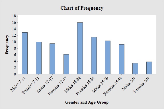
Construct a frequency bar graph.
a.
Answer to Problem 25E
Output obtained from MINITAB software for the gender and age group is:
Explanation of Solution
Calculation:
The given information is a table representing the numbers of people in various gender and age categories who used a video game console.
Software procedure:
- Step by step procedure to draw the bar chart for gender and age group using MINITAB software.
- Choose Graph > Bar Chart.
- From Bars represent, choose unique values from table.
- Choose Simple.
- Click OK.
- In Graph variables, enter the column of Frequency.
- In Categorical variables, enter the column of Gender and Age Group.
- Click OK
Observation:
From the bar graph, it can be seen that Males 18-34 has the highest frequency.
b.
Construct a relative frequency distribution for the data.
b.
Answer to Problem 25E
The relative frequency distribution for the data is:
| Gender and Age Group | Relative Frequency |
| Males 2-11 | 0.139 |
| Females 2-11 | 0.108 |
| Males 12-17 | 0.102 |
| Females 12-17 | 0.066 |
| Males 18-34 | 0.172 |
| Females 18-34 | 0.124 |
| Males 35-49 | 0.111 |
| Females 35-49 | 0.099 |
| Males 50+ | 0.037 |
| Females 50+ | 0.042 |
Explanation of Solution
Calculation:
Relative frequency:
The general formula for the relative frequency is,
Therefore,
Similarly, the relative frequencies for the gender and age group are obtained below:
| Gender and Age Group | Frequency | Relative Frequency |
| Males 2-11 | 13 | |
| Females 2-11 | 10.1 | |
| Males 12-17 | 9.6 | |
| Females 12-17 | 6.2 | |
| Males 18-34 | 16.1 | |
| Females 18-34 | 11.6 | |
| Males 35-49 | 10.4 | |
| Females 35-49 | 9.3 | |
| Males 50+ | 3.5 | |
| Females 50+ | 3.9 | |
| Total | 93.7 |
c.
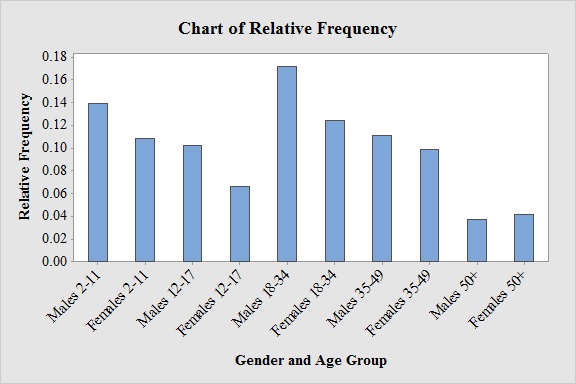
Construct a relative frequency bar graph for these data.
c.
Answer to Problem 25E
Output obtained from MINITAB software for the gender and age group is:
Explanation of Solution
Software procedure:
- Step by step procedure to draw the Bar chart for gender and age group using MINITAB software.
- Choose Graph > Bar Chart.
- From Bars represent, choose unique values from table.
- Choose Simple.
- Click OK.
- In Graph variables, enter the column of Relative Frequency.
- In Categorical variables, enter the column of Gender and Age Group.
- Click OK
Observation:
From the graph, it can be seen that most probable people in the various gender and age categories who used a video game console is Male 18-34 and the least probable people in the various gender and age categories who used a video game console is Male 50+.
d.
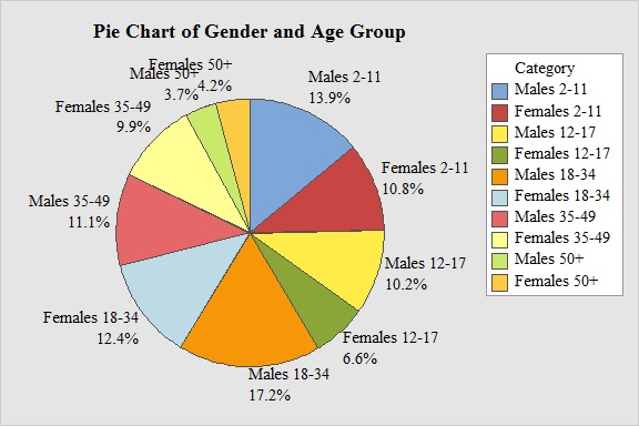
Construct a pie chart.
d.
Answer to Problem 25E
Output obtained from MINITAB software for gender and age group is:
Explanation of Solution
Calculation:
Software procedure:
- Step by step procedure to draw the bar chart for gender and age group using MINITAB software.
- Choose Graph > Pie Chart.
- Choose Chart values from table.
- Under categorical variable, select Gender and Age Group.
- Under Summary variables, select Relative Frequency.
- Click OK.
Observation:
There is about 17.2% of the people in Male 18-34 and the 3.7% of the people in Male 50+.
e.
Identify whether the statement “More than half of video gamers are male” is true or false.
e.
Answer to Problem 25E
The statement “More than half of video gamers are male” is true.
Explanation of Solution
From the pie chart, it can be seen that the percentage of male video gamers are
Hence, the statement “More than half of video gamers are male” is true.
Pie Chart:
It is a circle that divided into sectors one for each category.
g.
Identify whether the statement “More than 40% of video gamers are female” is true or false.
g.
Answer to Problem 25E
The statement “More than 40% of video gamers are female” is true.
Explanation of Solution
From the pie chart, it can be seen that the and the percentage of female video gamers are
Hence, the statement “More than 40% of video gamers are female” is true.
Pie Chart:
It is a circle that divided into sectors one for each category.
h.
Find the proportion of video gamers who are 35 or over.
h.
Answer to Problem 25E
The proportion of video gamers is 35 or over is 0.289.
Explanation of Solution
From the pie chart, it can be seen that the proportion of video gamers that are 35 or over aged are
Hence, the proportion of video gamers is 35 or over is 0.289.
Want to see more full solutions like this?
Chapter 2 Solutions
ALEKS 360 ESSENT. STAT ACCESS CARD


- State and prove the Morton's inequality Theorem 1.1 (Markov's inequality) Suppose that E|X|" 0, and let x > 0. Then, E|X|" P(|X|> x) ≤ x"arrow_forward(iii) If, in addition, X1, X2, ... Xn are identically distributed, then P(S|>x) ≤2 exp{-tx+nt²o}}.arrow_forward5. State space models Consider the model T₁ = Tt−1 + €t S₁ = 0.8S-4+ Nt Y₁ = T₁ + S₁ + V₂ where (+) Y₁,..., Y. ~ WN(0,σ²), nt ~ WN(0,σ2), and (V) ~ WN(0,0). We observe data a. Write the model in the standard (matrix) form of a linear Gaussian state space model. b. Does lim+++∞ Var (St - St|n) exist? If so, what is its value? c. Does lim∞ Var(T₁ — Ît\n) exist? If so, what is its value?arrow_forward
- Let X represent the full height of a certain species of tree. Assume that X has a normal probability distribution with mean 203.8 ft and standard deviation 43.8 ft. You intend to measure a random sample of n = 211trees. The bell curve below represents the distribution of these sample means. The scale on the horizontal axis (each tick mark) is one standard error of the sampling distribution. Complete the indicated boxes, correct to two decimal places. Image attached. I filled in the yellow boxes and am not sure why they are wrong. There are 3 yellow boxes filled in with values 206.82; 209.84; 212.86.arrow_forwardCould you please answer this question using excel.Thanksarrow_forwardQuestions An insurance company's cumulative incurred claims for the last 5 accident years are given in the following table: Development Year Accident Year 0 2018 1 2 3 4 245 267 274 289 292 2019 255 276 288 294 2020 265 283 292 2021 263 278 2022 271 It can be assumed that claims are fully run off after 4 years. The premiums received for each year are: Accident Year Premium 2018 306 2019 312 2020 318 2021 326 2022 330 You do not need to make any allowance for inflation. 1. (a) Calculate the reserve at the end of 2022 using the basic chain ladder method. (b) Calculate the reserve at the end of 2022 using the Bornhuetter-Ferguson method. 2. Comment on the differences in the reserves produced by the methods in Part 1.arrow_forward
- Calculate the correlation coefficient r, letting Row 1 represent the x-values and Row 2 the y-values. Then calculate it again, letting Row 2 represent the x-values and Row 1 the y-values. What effect does switching the variables have on r? Row 1 Row 2 13 149 25 36 41 60 62 78 S 205 122 195 173 133 197 24 Calculate the correlation coefficient r, letting Row 1 represent the x-values and Row 2 the y-values. r=0.164 (Round to three decimal places as needed.) S 24arrow_forwardThe number of initial public offerings of stock issued in a 10-year period and the total proceeds of these offerings (in millions) are shown in the table. The equation of the regression line is y = 47.109x+18,628.54. Complete parts a and b. 455 679 499 496 378 68 157 58 200 17,942|29,215 43,338 30,221 67,266 67,461 22,066 11,190 30,707| 27,569 Issues, x Proceeds, 421 y (a) Find the coefficient of determination and interpret the result. (Round to three decimal places as needed.)arrow_forwardQuestions An insurance company's cumulative incurred claims for the last 5 accident years are given in the following table: Development Year Accident Year 0 2018 1 2 3 4 245 267 274 289 292 2019 255 276 288 294 2020 265 283 292 2021 263 278 2022 271 It can be assumed that claims are fully run off after 4 years. The premiums received for each year are: Accident Year Premium 2018 306 2019 312 2020 318 2021 326 2022 330 You do not need to make any allowance for inflation. 1. (a) Calculate the reserve at the end of 2022 using the basic chain ladder method. (b) Calculate the reserve at the end of 2022 using the Bornhuetter-Ferguson method. 2. Comment on the differences in the reserves produced by the methods in Part 1.arrow_forward
- Use the accompanying Grade Point Averages data to find 80%,85%, and 99%confidence intervals for the mean GPA. view the Grade Point Averages data. Gender College GPAFemale Arts and Sciences 3.21Male Engineering 3.87Female Health Science 3.85Male Engineering 3.20Female Nursing 3.40Male Engineering 3.01Female Nursing 3.48Female Nursing 3.26Female Arts and Sciences 3.50Male Engineering 3.00Female Arts and Sciences 3.13Female Nursing 3.34Female Nursing 3.67Female Education 3.45Female Engineering 3.17Female Health Science 3.28Female Nursing 3.25Male Engineering 3.72Female Arts and Sciences 2.68Female Nursing 3.40Female Health Science 3.76Female Arts and Sciences 3.72Female Education 3.44Female Arts and Sciences 3.61Female Education 3.29Female Nursing 3.20Female Education 3.80Female Business 3.26Male…arrow_forwardBusiness Discussarrow_forwardCould you please answer this question using excel. For 1a) I got 84.75 and for part 1b) I got 85.33 and was wondering if you could check if my answers were correct. Thanksarrow_forward
 MATLAB: An Introduction with ApplicationsStatisticsISBN:9781119256830Author:Amos GilatPublisher:John Wiley & Sons Inc
 Probability and Statistics for Engineering and th...StatisticsISBN:9781305251809Author:Jay L. DevorePublisher:Cengage Learning
 Statistics for The Behavioral Sciences (MindTap C...StatisticsISBN:9781305504912Author:Frederick J Gravetter, Larry B. WallnauPublisher:Cengage Learning
 Elementary Statistics: Picturing the World (7th E...StatisticsISBN:9780134683416Author:Ron Larson, Betsy FarberPublisher:PEARSON
 The Basic Practice of StatisticsStatisticsISBN:9781319042578Author:David S. Moore, William I. Notz, Michael A. FlignerPublisher:W. H. Freeman
 Introduction to the Practice of StatisticsStatisticsISBN:9781319013387Author:David S. Moore, George P. McCabe, Bruce A. CraigPublisher:W. H. Freeman