
Videos
(a)
To graph: A stem-and-leaf plot for the data of the age distribution.
(a)
Explanation of Solution
The data shows the ages of 50 drivers arrested while driver under the influence of alcohol.
Graph: To construct stem-and-leaf plot by using the Minitab, the steps are as follows:
Step 1: Enter the data in C1.
Step 2: Go to Graph > Stem-and-Leaf plot and select ‘C1’ in Graph variable.
Step 3: Click on OK.
The Stem-and-Leaf plot for these data is obtained as:
| Stem-and-leaf of the age distribution N = 50 | ||
| 1 | 6 8 | |
| 2 | 0 1 1 2 2 2 3 4 4 5 6 6 6 7 7 7 9 | |
| 3 | 0 0 1 1 2 3 4 4 5 5 6 7 8 9 | |
| 4 | 0 0 1 3 5 6 7 7 9 9 | |
| 5 | 1 3 5 6 8 | |
| 6 | 3 4 | |
(b)
To find: The frequency table for the data..
(b)
Answer to Problem 8CR
Solution: The complete frequency table is as:
| Class Limits | Class boundaries | Midpoints | Frequency | Relative Frequency | Cumulative Frequency |
| 16-22 | 15.5-22.5 | 19 | 8 | 0.16 | 8 |
| 23-29 | 22.5-29.5 | 26 | 11 | 0.22 | 19 |
| 30-36 | 29.5-36.5 | 33 | 11 | 0.22 | 30 |
| 37-43 | 36.5-43.5 | 40 | 7 | 0.14 | 37 |
| 44-50 | 43.5-50.5 | 47 | 6 | 0.12 | 43 |
| 51-57 | 50.5-57.5 | 54 | 4 | 0.08 | 47 |
| 58-64 | 57.5-64.5 | 61 | 3 | 0.06 | 50 |
Explanation of Solution
Calculation: To find the class width for the whole data of 50 values, it is observed that largest value of the data set is 64 and the smallest value is 16 in the data. Using 7 classes, the class width calculated in the following way:
The value is round up to the nearest whole number. Hence, the class width of the data set is 7. The class width for the data is 7 and the lowest data value (16) will be the lower class limit of the first class. Because the class width is 7, it must add 7 to the lowest class limit in the first class to find the lowest class limit in the second class. There are 7 desired classes. Hence, the class limits are 16-22, 23-29, 30-36, 37-43, 44-50, 51-57, and 58-64. Now, to find the class boundaries subtract 0.5 from lower limit of every class and add 0.5 to the upper limit of the every class interval. Hence, the class boundaries are 15.5-22.5, 22.5-29.5, 29.5-36.5, 36.5-43.5, 43.5-50.5, 50.5-57.5, and 57.5-64.5.
Next to find the midpoint of the class is calculated by using formula,
Midpoint of first class is calculated as:
The frequencies for respective classes are 8, 11, 11, 7, 6, 4 and 3.
Relative frequency is calculated by using the formula,
The frequency for 1st class is 8 and total frequencies are 50 so the relative frequency is
The calculated frequency table is as follows:
| Class limits | Class boundaries | midpoints | Frequency | Relative Frequency | Cumulative Frequency |
| 16-22 | 15.5-22.5 | 19 | 8 | 0.16 | 8 |
| 23-29 | 22.5-29.5 | 26 | 11 | 0.22 | |
| 30-36 | 29.5-36.5 | 33 | 11 | 0.22 | |
| 37-43 | 36.5-43.5 | 40 | 7 | 0.14 | |
| 44-50 | 43.5-50.5 | 47 | 6 | 0.12 | |
| 51-57 | 50.5-57.5 | 54 | 4 | 0.08 | |
| 58-64 | 57.5-64.5 | 61 | 3 | 0.06 |
Interpretation: Hence, the complete frequency table is as:
| Class limits | Class boundaries | Midpoints | Frequency | Relative Frequency | Cumulative Frequency |
| 16-22 | 15.5-22.5 | 19 | 8 | 0.16 | 8 |
| 23-29 | 22.5-29.5 | 26 | 11 | 0.22 | |
| 30-36 | 29.5-36.5 | 33 | 11 | 0.22 | |
| 37-43 | 36.5-43.5 | 40 | 7 | 0.14 | |
| 44-50 | 43.5-50.5 | 47 | 6 | 0.12 | |
| 51-57 | 50.5-57.5 | 54 | 4 | 0.08 | |
| 58-64 | 57.5-64.5 | 61 | 3 | 0.06 |
(c)
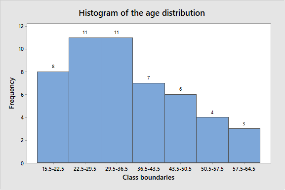
To graph: A histogram for the data of the age distribution.
(c)
Explanation of Solution
The data shows the ages of 50 drivers arrested while driver under the influence of alcohol.
Graph: To construct the histogram by using the MINITAB, the steps are as follows:
Step 1: Enter the class boundaries in C1 and frequency in C2.
Step 2: Go to Graph > Histogram > Simple.
Step 3: Enter C1 in Graph variable then go to Data options > Frequency > C2.
Step 4: Click on OK.
The obtained histogram is
(d)
The shape of the histogram of age distribution..
(d)
Answer to Problem 8CR
Solution: The shape of histogram of age distribution is skewed to the right.
Explanation of Solution
A right-skewed distribution has a long right tail. Right-skewed distributions are also called positive-skew distributions. That’s because there is a long tail in the positive direction on the number line.
From above histogram, there are two class boundaries (22.5-29.5 and 29.5-36) have higher frequencies 11 on left side and most of the data values fall on the left side of the graph. The data to lean towards right side of the graph and also there is tail on right side.
Hence, the shape of histogram of age distribution is skewed to the right.
Want to see more full solutions like this?
Chapter 2 Solutions
UNDERSTANDING BASIC STAT LL BUND >A< F


- Negate the following compound statement using De Morgans's laws.arrow_forwardQuestion 6: Negate the following compound statements, using De Morgan's laws. A) If Alberta was under water entirely then there should be no fossil of mammals.arrow_forwardNegate the following compound statement using De Morgans's laws.arrow_forward
- Characterize (with proof) all connected graphs that contain no even cycles in terms oftheir blocks.arrow_forwardLet G be a connected graph that does not have P4 or C3 as an induced subgraph (i.e.,G is P4, C3 free). Prove that G is a complete bipartite grapharrow_forwardProve sufficiency of the condition for a graph to be bipartite that is, prove that if G hasno odd cycles then G is bipartite as follows:Assume that the statement is false and that G is an edge minimal counterexample. That is, Gsatisfies the conditions and is not bipartite but G − e is bipartite for any edge e. (Note thatthis is essentially induction, just using different terminology.) What does minimality say aboutconnectivity of G? Can G − e be disconnected? Explain why if there is an edge between twovertices in the same part of a bipartition of G − e then there is an odd cyclearrow_forward
- Let G be a connected graph that does not have P4 or C4 as an induced subgraph (i.e.,G is P4, C4 free). Prove that G has a vertex adjacent to all othersarrow_forwardWe consider a one-period market with the following properties: the current stock priceis S0 = 4. At time T = 1 year, the stock has either moved up to S1 = 8 (with probability0.7) or down towards S1 = 2 (with probability 0.3). We consider a call option on thisstock with maturity T = 1 and strike price K = 5. The interest rate on the money marketis 25% yearly.(a) Find the replicating portfolio (φ, ψ) corresponding to this call option.(b) Find the risk-neutral (no-arbitrage) price of this call option.(c) We now consider a put option with maturity T = 1 and strike price K = 3 onthe same market. Find the risk-neutral price of this put option. Reminder: A putoption gives you the right to sell the stock for the strike price K.1(d) An investor with initial capital X0 = 0 wants to invest on this market. He buysα shares of the stock (or sells them if α is negative) and buys β call options (orsells them is β is negative). He invests the cash balance on the money market (orborrows if the amount is…arrow_forwardDetermine if the two statements are equivalent using a truth tablearrow_forward
- Question 4: Determine if pair of statements A and B are equivalent or not, using truth table. A. (~qp)^~q в. р л~9arrow_forwardDetermine if the two statements are equalivalent using a truth tablearrow_forwardQuestion 3: p and q represent the following simple statements. p: Calgary is the capital of Alberta. A) Determine the value of each simple statement p and q. B) Then, without truth table, determine the va q: Alberta is a province of Canada. for each following compound statement below. pvq р^~q ~рл~q ~q→ p ~P~q Pq b~ (d~ ← b~) d~ (b~ v d) 0 4arrow_forward
 Glencoe Algebra 1, Student Edition, 9780079039897...AlgebraISBN:9780079039897Author:CarterPublisher:McGraw Hill