Refer to the North Valley Real Estate data that reports information on homes sold during the last year. For the variable price, select an appropriate class interval and organize the selling prices into a frequency distribution. Write a brief report summarizing your findings. Be sure to answer the following questions in your report.
- a. Around what values of price do the data tend to cluster?
- b. Based on the frequency distribution, what is the typical selling price in the first class? What is the typical selling price in the last class?
- c. Draw a cumulative relative frequency distribution. Using this distribution, fifty percent of the homes sold for what price or less? Estimate the lower price of the top ten percent of homes sold. About what percent of the homes sold for less than $300,000?
- d. Refer to the variable bedrooms. Draw a bar chart showing the number of homes sold with 2, 3, 4 or more bedrooms. Write a description of the distribution.
a.
Find an appropriate class interval.
Create a frequency distribution for the selling prices and explain the results.
At what values of price the data tend to cluster.
Answer to Problem 51DA
The frequency distribution for the selling price is given below:
|
Selling price (1,000’s) | Frequency |
Cumulative frequency |
| 120-240 | 26 | 26 |
| 240-360 | 36 | |
| 360-480 | 27 | |
| 480-600 | 7 | |
| 600-720 | 4 | |
| 720-840 | 2 | |
| 840-960 | 3 | |
| Total | 105 |
Explanation of Solution
Selection of number of classes:
“2 to the k rule” suggests that the number of classes is the smallest value of k, where
It is given that the data set consists of 105 observations. The value of k can be obtained as follows:
Here,
Therefore, the number of classes for the given data set is 7.
From the data set North Valley Real Estate Data, the maximum and minimum values are 919,480 and 167,962, respectively.
The formula for the class interval is given as follows:
Where, i is the class interval and k is the number of classes.
Therefore, the class interval for the given data can be obtained as follows:
In practice, the class interval size is usually rounded up to some convenient number. Therefore, the reasonable class interval is 120,000.
Frequency distribution:
The frequency table is a collection of mutually exclusive and exhaustive classes, which shows the number of observations in each class.
Since the minimum value is 167,962 and the class interval is 120,000, the first class would be 120,000-240,000 or 160,000-280,000. Here, the first one is preferred as the first class of the frequency distribution. The frequency distribution for the selling price can be constructed as follows:
|
Selling price (1,000’s) | Frequency |
Cumulative frequency |
| 120-240 | 26 | 26 |
| 240-360 | 36 | |
| 360-480 | 27 | |
| 480-600 | 7 | |
| 600-720 | 4 | |
| 720-840 | 2 | |
| 840-960 | 3 | |
| Total | 105 |
From the above table, 89 out of 105 homes are sold between $120,000 and $480,000.
b.
Find the typical selling in first class.
Find the typical selling in last class.
Answer to Problem 51DA
The typical selling price of first class is $180,000.
The typical selling price of last class is $900,000.
Explanation of Solution
The lower and upper limits of the first class are $120,000 and $240,000.
The typical selling price of first class is calculated as follows:
Thus, typical selling price of first class is $180,000.
The lower and upper limits of the last class are $840,000 and $960,000.
The typical selling price of last class is calculated as follows:
Thus, typical selling price of last class is $900,000.
c.
Create a cumulative relative frequency polygon for the frequency distribution.
Identify the price for which less than 50% of the homes are sold.
Find the lower price of the top 10% of homes are sold.
About what percentage of homes are sold for less than $300,000.
Answer to Problem 51DA
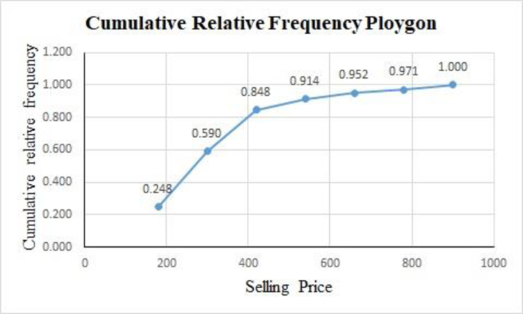
The cumulative frequency polygon for the given data is as follows:

There are 50% of the homes sold approximately less than $254,000.
The top 10% of homes are sold for at least $520,000.
There are 59% of homes sold for less than $300,000.
Explanation of Solution
For the given data set, the cumulative relative frequency table with midpoints of classes is obtained as follows:
|
Selling price (1,000’s) | Midpoint |
Cumulative frequency |
Relative cumulative frequency |
| 120-240 | 26 | ||
| 240-360 | 62 | ||
| 360-480 | 89 | ||
| 480-600 | 96 | ||
| 600-720 | 100 | ||
| 720-840 | 102 | ||
| 840-960 | 105 |
The cumulative relative frequency polygon for the given data can be drawn using EXCEL.
Step-by-step procedure to obtain the frequency polygon using EXCEL is as follows:
- Enter the column of midpoints along with the cumulative relative frequency column.
- Select the total data range with labels.
- Go to Insert > Charts > line chart.
- Select the appropriate line chart.
- Click OK.
From the above cumulative relative frequency polygon, 50% of the homes are sold approximately less than $254,000.
The top 10% of homes are sold for at least $520,000.
There are 59% of homes sold for less than $300,000.
d.
Create a bar chart for the number of bedrooms for the variable bedrooms.
Answer to Problem 51DA
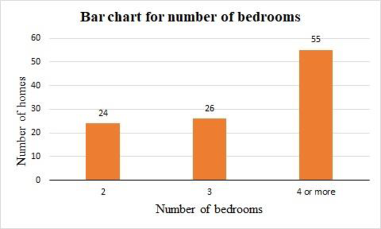
The bar chart for the number of bedrooms for the variable bedrooms is as follows:

Explanation of Solution
For the variable bedrooms, the frequency table is obtained as follows:
|
Number of bedrooms | Frequency |
| 2 | 24 |
| 3 | 26 |
| 4 or more | 55 |
| Total | 105 |
The bar chart for the given data can be drawn using EXCEL.
Step-by-step procedure to obtain the bar chart using EXCEL is as follows:
- Enter the column of bedrooms along with the frequency column.
- Select the total data range with labels.
- Go to Insert > Charts > bar chart.
- Select the appropriate bar chart.
- Click OK.
From the above bar chart, the highest frequency occurred in the last category, the shape of the distribution is negatively skewed.
Want to see more full solutions like this?
Chapter 2 Solutions
Gen Combo Ll Statistical Techniques In Business And Economics; Connect Ac
- Good explanation it sure experts solve itarrow_forwardBest explains it not need guidelines okkarrow_forwardActiv Determine compass error using amplitude (Sun). Minimum number of times that activity should be performed: 3 (1 each phase) Sample calculation (Amplitude- Sun): On 07th May 2006 at Sunset, a vessel in position 10°00'N 010°00'W observed the Sun bearing 288° by compass. Find the compass error. LMT Sunset: LIT: (+) 00d 07d 18h 00h 13m 40m UTC Sunset: 07d 18h 53m (added- since longitude is westerly) Declination (07d 18h): N 016° 55.5' d (0.7): (+) 00.6' Declination Sun: N 016° 56.1' Sin Amplitude = Sin Declination/Cos Latitude = Sin 016°56.1'/ Cos 10°00' = 0.295780189 Amplitude=W17.2N (The prefix of amplitude is named easterly if body is rising, and westerly if body is setting. The suffix is named same as declination) True Bearing=287.2° Compass Bearing= 288.0° Compass Error = 0.8° Westarrow_forward
- Only sure experts solve it correct complete solutions okkarrow_forward13. In 2000, two organizations conducted surveys to ascertain the public's opinion on banning gay men from serving in leadership roles in the Boy Scouts.• A Pew poll asked respondents whether they agreed with "the recent decision by the Supreme Court" that "the Boy Scouts of America have a constitutional right to block gay men from becoming troop leaders."A Los Angeles Times poll asked respondents whether they agreed with the following statement: "A Boy Scout leader should be removed from his duties as a troop leader if he is found out to be gay, even if he is considered by the Scout organization to be a model Boy Scout leader."One of these polls found 36% agreement; the other found 56% agreement. Which of the following statements is true?A) The Pew poll found 36% agreement, and the Los Angeles Times poll found 56% agreement.B) The Pew poll includes a leading question, while the Los Angeles Times poll uses neutral wording.C) The Los Angeles Times Poll includes a leading question, while…arrow_forwardAnswer questions 2arrow_forward
- (c) Give an example where PLANBAC)= PCAPCBIPCC), but the sets are not pairwise independentarrow_forwardScrie trei multiplii comuni pentru numerele 12 și 1..arrow_forwardIntroduce yourself and describe a time when you used data in a personal or professional decision. This could be anything from analyzing sales data on the job to making an informed purchasing decision about a home or car. Describe to Susan how to take a sample of the student population that would not represent the population well. Describe to Susan how to take a sample of the student population that would represent the population well. Finally, describe the relationship of a sample to a population and classify your two samples as random, systematic, cluster, stratified, or convenience.arrow_forward
- 1.2.17. (!) Let G,, be the graph whose vertices are the permutations of (1,..., n}, with two permutations a₁, ..., a,, and b₁, ..., b, adjacent if they differ by interchanging a pair of adjacent entries (G3 shown below). Prove that G,, is connected. 132 123 213 312 321 231arrow_forwardYou are planning an experiment to determine the effect of the brand of gasoline and the weight of a car on gas mileage measured in miles per gallon. You will use a single test car, adding weights so that its total weight is 3000, 3500, or 4000 pounds. The car will drive on a test track at each weight using each of Amoco, Marathon, and Speedway gasoline. Which is the best way to organize the study? Start with 3000 pounds and Amoco and run the car on the test track. Then do 3500 and 4000 pounds. Change to Marathon and go through the three weights in order. Then change to Speedway and do the three weights in order once more. Start with 3000 pounds and Amoco and run the car on the test track. Then change to Marathon and then to Speedway without changing the weight. Then add weights to get 3500 pounds and go through the three gasolines in the same order.Then change to 4000 pounds and do the three gasolines in order again. Choose a gasoline at random, and run the car with this gasoline at…arrow_forwardAP1.2 A child is 40 inches tall, which places her at the 90th percentile of all children of similar age. The heights for children of this age form an approximately Normal distribution with a mean of 38 inches. Based on this information, what is the standard deviation of the heights of all children of this age? 0.20 inches (c) 0.65 inches (e) 1.56 inches 0.31 inches (d) 1.21 inchesarrow_forward
 Holt Mcdougal Larson Pre-algebra: Student Edition...AlgebraISBN:9780547587776Author:HOLT MCDOUGALPublisher:HOLT MCDOUGAL
 Glencoe Algebra 1, Student Edition, 9780079039897...AlgebraISBN:9780079039897Author:CarterPublisher:McGraw Hill
 Big Ideas Math A Bridge To Success Algebra 1: Stu...AlgebraISBN:9781680331141Author:HOUGHTON MIFFLIN HARCOURTPublisher:Houghton Mifflin Harcourt
 Functions and Change: A Modeling Approach to Coll...AlgebraISBN:9781337111348Author:Bruce Crauder, Benny Evans, Alan NoellPublisher:Cengage Learning


