
Videos
a.
Obtain a frequency distribution for the variable Team salary.
Find the typical salary for a team.
Find the
a.
Answer to Problem 52DA
The frequency distribution for the salary is given below:
| Salary $1,000,000’s | Number of teams | Cumulative frequency |
| 60-100 | 10 | 10 |
| 100-140 | 12 | 22 |
| 140-180 | 6 | 28 |
| 180-220 | 1 | 29 |
| 220-260 | 1 | 30 |
| Total | 30 |
The typical salary of a team is from 100 to 400 million dollars.
The range of the salaries is 200 million dollars.
Explanation of Solution
Selection of number of classes:
“2 to the k rule” suggests that the number of classes is the smallest value of k, where
It is given that the data set consists of 30 observations. The value of k can be obtained as follows:
Here,
Therefore, the number of classes for the given data set is 5.
From the data set Team salary, the maximum and minimum values are 230.4 and 65.8, respectively.
The formula for the class interval is given as follows:
Where, i is the class interval and k is the number of classes.
Therefore, the class interval for the given data can be obtained as follows:
In practice, the class interval size is usually rounded up to some convenient number. Therefore, the reasonable class interval is 40.
Frequency distribution:
The frequency table is a collection of mutually exclusive and exhaustive classes, which shows the number of observations in each class.
Since the minimum value is 65.8 and the class interval is 40, the first class would be 60–100. The frequency distribution for salary can be constructed as follows:
| Salary $1,000,000’s | Number of teams | Cumulative frequency |
| 60-100 | 10 | 10 |
| 100-140 | 12 | |
| 140-180 | 6 | |
| 180-220 | 1 | |
| 220-260 | 1 | |
| Total | 30 |
From the above frequency distribution, the typical salary of a team is from 100 to 400 million dollars.
The range of the salaries is from 60 to 260 million dollars. Thus, range of the salaries is 200 million dollars.
b.
Make a comment on shape of the distribution.
Check whether there are any teams that have a salary out of the line with the others.
b.
Answer to Problem 52DA
The distribution of salaries is positively skewed.
There are two teams with salaries much higher than the remaining 28 team salaries.
Explanation of Solution
From the frequency distribution in Part (a), 22 out of 30 teams fall in first and second classes. Therefore, the distribution of salaries is positively skewed.
There are two teams with salaries much higher than the remaining 28 team salaries. These two teams have a salary out of the line with the others.
c.
Create a cumulative relative frequency
Identify the amount that is less than for the 40% of the team’s salary.
Find the number of teams that have a total salary of more than $220 million.
c.
Answer to Problem 52DA
The cumulative frequency polygon for the given data is as follows:
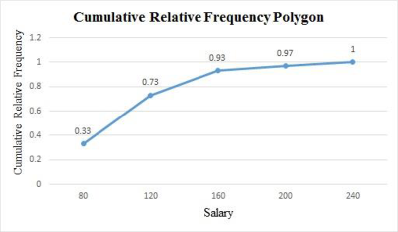
There are 40% of the teams that have salary less than 90 million dollars.
There is only one team that is getting salary more than 220 million dollars.
Explanation of Solution
For the given data set, the cumulative relative frequency table with midpoints of classes is obtained as follows:
| Salary$1,000,000’s | Midpoint | Cumulative frequency | Relative cumulative frequency |
| 60-100 | 10 | ||
| 100-140 | 22 | ||
| 140-180 | 28 | ||
| 180-220 | 29 | ||
| 220-260 | 30 |
The cumulative relative frequency polygon for the given data can be drawn using EXCEL.
Step-by-step procedure to obtain the frequency polygon using EXCEL is as follows:
- Enter the column of midpoints along with the cumulative relative frequency column.
- Select the total data range with labels.
- Go to Insert > Charts > line chart.
- Select the appropriate line chart.
- Click OK.
From the above cumulative relative frequency polygon, 40% of the teams have salary less than 90 million dollars.
There are 3% of the teams that get salary more than 220 million dollars. In the given data, 3% of teams are equal to 1 team. Thus, only one team is getting salary more than 220 million dollars.
Want to see more full solutions like this?
Chapter 2 Solutions
Gen Combo Ll Statistical Techniques In Business And Economics; Connect Ac


- A company found that the daily sales revenue of its flagship product follows a normal distribution with a mean of $4500 and a standard deviation of $450. The company defines a "high-sales day" that is, any day with sales exceeding $4800. please provide a step by step on how to get the answers in excel Q: What percentage of days can the company expect to have "high-sales days" or sales greater than $4800? Q: What is the sales revenue threshold for the bottom 10% of days? (please note that 10% refers to the probability/area under bell curve towards the lower tail of bell curve) Provide answers in the yellow cellsarrow_forwardFind the critical value for a left-tailed test using the F distribution with a 0.025, degrees of freedom in the numerator=12, and degrees of freedom in the denominator = 50. A portion of the table of critical values of the F-distribution is provided. Click the icon to view the partial table of critical values of the F-distribution. What is the critical value? (Round to two decimal places as needed.)arrow_forwardA retail store manager claims that the average daily sales of the store are $1,500. You aim to test whether the actual average daily sales differ significantly from this claimed value. You can provide your answer by inserting a text box and the answer must include: Null hypothesis, Alternative hypothesis, Show answer (output table/summary table), and Conclusion based on the P value. Showing the calculation is a must. If calculation is missing,so please provide a step by step on the answers Numerical answers in the yellow cellsarrow_forward
 Big Ideas Math A Bridge To Success Algebra 1: Stu...AlgebraISBN:9781680331141Author:HOUGHTON MIFFLIN HARCOURTPublisher:Houghton Mifflin Harcourt
 Glencoe Algebra 1, Student Edition, 9780079039897...AlgebraISBN:9780079039897Author:CarterPublisher:McGraw Hill
 Holt Mcdougal Larson Pre-algebra: Student Edition...AlgebraISBN:9780547587776Author:HOLT MCDOUGALPublisher:HOLT MCDOUGAL