
Videos
To find: A
Answer to Problem 178E
Solution: For the pair of variables: (EdCollege, Female), the coefficient of determination value is
For the pair of variables: (EdCollege, Age 18-24), the coefficient of determination value is
For the pair of variables: (EdCollege, Age 25-34), the coefficient of determination value is
Explanation of Solution
Given: The data of 50 states with variables related to health conditions and risk behavior as well as demographic information is provided in the question.
| State | Age18_24 | Age25_34 | Female | EdCollege |
| Alabama | 13.0 | 17.1 | 52.3 | 19.7 |
| Alaska | 14.6 | 20.7 | 48.2 | 23.7 |
| Arizona | 12.5 | 19.2 | 50.4 | 23.7 |
| Arkansas | 12.6 | 17.7 | 51.7 | 17.4 |
| California | 13.4 | 19.3 | 50.4 | 27.0 |
| Colorado | 12.7 | 18.2 | 49.9 | 32.6 |
| Connecticut | 12.3 | 15.2 | 51.9 | 32.5 |
| Delaware | 12.1 | 16.8 | 52.3 | 25.3 |
| District of Columbia | 13.9 | 23.0 | 53.7 | 45.2 |
| Florida | 11.3 | 16.2 | 51.4 | 23.8 |
| Georgia | 13.4 | 18.8 | 51.4 | 24.6 |
| Guam | 16.9 | 19.6 | 49.0 | 26.0 |
| Hawaii | 11.9 | 18.8 | 50.0 | 26.7 |
| Idaho | 14.1 | 18.4 | 50.2 | 21.7 |
| Illinois | 13.2 | 18.0 | 51.3 | 27.8 |
| Indiana | 13.4 | 17.1 | 51.3 | 20.5 |
| Iowa | 13.6 | 16.0 | 51.1 | 22.6 |
| Kansas | 14.0 | 17.5 | 50.9 | 26.5 |
| Kentucky | 12.5 | 17.3 | 51.6 | 18.7 |
| Louisiana | 13.8 | 18.6 | 52.2 | 18.9 |
| Maine | 11.1 | 14.3 | 51.8 | 24.5 |
| Maryland | 12.3 | 17.3 | 52.3 | 32.8 |
| Massachusetts | 12.7 | 16.6 | 52.1 | 35.4 |
| Michigan | 13.1 | 15.7 | 51.4 | 22.8 |
| Minnesota | 12.8 | 17.4 | 50.7 | 28.8 |
| Mississippi | 14.4 | 17.9 | 52.3 | 17.5 |
| Missouri | 12.9 | 17.2 | 51.8 | 23.0 |
| Montana | 12.9 | 15.8 | 50.3 | 25.1 |
| Nebraska | 14.2 | 17.4 | 50.9 | 25.2 |
| Nevada | 11.7 | 19.5 | 49.4 | 19.9 |
| New Hampshire | 12.4 | 14.5 | 51.2 | 30.2 |
| New Jersey | 11.3 | 16.4 | 51.6 | 32.3 |
| New Mexico | 13.1 | 18.6 | 51.0 | 22.7 |
| New York | 12.5 | 17.4 | 52.1 | 29.9 |
| North Carolina | 12.9 | 17.2 | 51.7 | 23.8 |
| North Dakota | 16.8 | 16.8 | 50.0 | 23.6 |
| Ohio | 12.3 | 16.6 | 51.9 | 22.3 |
| Oklahoma | 13.8 | 18.2 | 51.2 | 20.4 |
| Oregon | 12.2 | 16.3 | 50.8 | 26.1 |
| Pennsylvania | 12.3 | 15.6 | 52.0 | 24.5 |
| Puerto Rico | 14.6 | 19.2 | 53.1 | 19.4 |
| Rhode Island | 13.2 | 15.9 | 52.2 | 27.5 |
| South Carolina | 12.8 | 17.1 | 52.1 | 21.8 |
| South Dakota | 13.9 | 17.0 | 50.4 | 22.9 |
| Tennessee | 12.1 | 17.3 | 51.9 | 20.9 |
| Texas | 13.9 | 19.7 | 50.6 | 23.1 |
| Utah | 17.2 | 22.8 | 50.1 | 25.4 |
| Vermont | 13.2 | 14.2 | 51.3 | 30.2 |
| Virginia | 12.9 | 17.2 | 51.3 | 30.9 |
Calculation: From the given data set consider the following three pair of variables.
1. EdCollege and Female
2. EdCollege and Age 18-24
3. EdCollege and Age 25-34
Now, construct the scatterplot with fitted linear regression line for each pair of variables.
Use Minitab to get the required result.
To draw the scatterplot of the provided data, below mentioned steps are followed in Minitab.
Step 1: Enter the data into Minitab worksheet.
Step 2: Go to Graph, select scatterplot and linear regression and click OK.
Step 3: Select the data variable column and click on Scale.
Step 4: Check minor ticks under Y Scale Low and X Scale Low and then click OK.
The obtained scatterplot of EdCollege and Female is shown below:
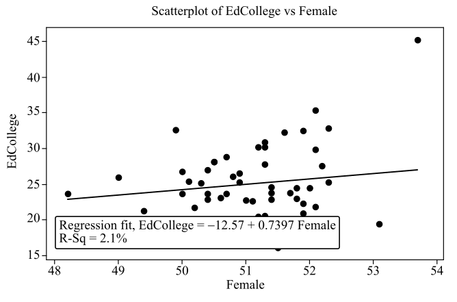
From the above plot we observe that there is a low positive relation between the two variables female and EdCollege.
The regression fit for the data is
The obtained scatterplot of EdCollege and Age 18-24 is shown below.
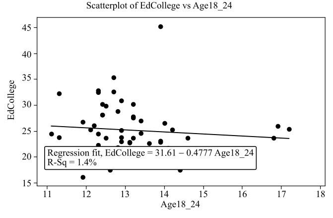
From the above plot we observe that there is a low negative relation between the two variables Age 18-24 and EdCollege. The regression fit for the data is
The obtained scatterplot of EdCollege and Age 25-34 is shown below.
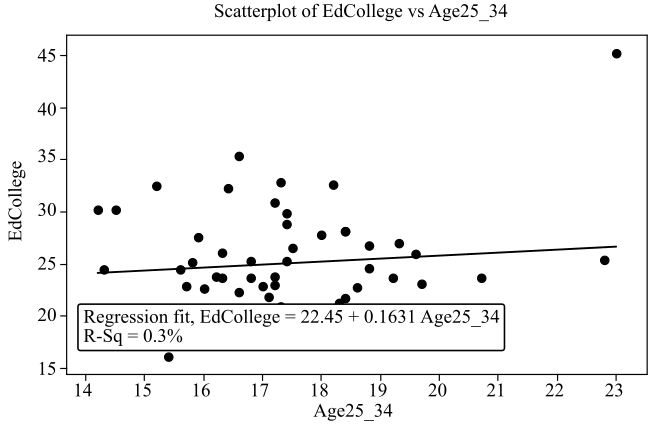
From the above plot we observe that there is a low positive relation between the two variables Age 25-34 and EdCollege.
The regression fit for the data is
Interpretation: Consider the first pair of variables, EdCollege and Female. The coefficient of determination value is
Consider second pair of variables, EdCollege and Age 18-24. The coefficient of determination value is
Consider third pair of variables, EdCollege and Age 25-34. The coefficient of determination value is
Want to see more full solutions like this?
Chapter 2 Solutions
EBK INTRODUCTION TO THE PRACTICE OF STA


- For a binary asymmetric channel with Py|X(0|1) = 0.1 and Py|X(1|0) = 0.2; PX(0) = 0.4 isthe probability of a bit of “0” being transmitted. X is the transmitted digit, and Y is the received digit.a. Find the values of Py(0) and Py(1).b. What is the probability that only 0s will be received for a sequence of 10 digits transmitted?c. What is the probability that 8 1s and 2 0s will be received for the same sequence of 10 digits?d. What is the probability that at least 5 0s will be received for the same sequence of 10 digits?arrow_forwardV2 360 Step down + I₁ = I2 10KVA 120V 10KVA 1₂ = 360-120 or 2nd Ratio's V₂ m 120 Ratio= 360 √2 H I2 I, + I2 120arrow_forwardQ2. [20 points] An amplitude X of a Gaussian signal x(t) has a mean value of 2 and an RMS value of √(10), i.e. square root of 10. Determine the PDF of x(t).arrow_forward
- In a network with 12 links, one of the links has failed. The failed link is randomlylocated. An electrical engineer tests the links one by one until the failed link is found.a. What is the probability that the engineer will find the failed link in the first test?b. What is the probability that the engineer will find the failed link in five tests?Note: You should assume that for Part b, the five tests are done consecutively.arrow_forwardProblem 3. Pricing a multi-stock option the Margrabe formula The purpose of this problem is to price a swap option in a 2-stock model, similarly as what we did in the example in the lectures. We consider a two-dimensional Brownian motion given by W₁ = (W(¹), W(2)) on a probability space (Q, F,P). Two stock prices are modeled by the following equations: dX = dY₁ = X₁ (rdt+ rdt+0₁dW!) (²)), Y₁ (rdt+dW+0zdW!"), with Xo xo and Yo =yo. This corresponds to the multi-stock model studied in class, but with notation (X+, Y₁) instead of (S(1), S(2)). Given the model above, the measure P is already the risk-neutral measure (Both stocks have rate of return r). We write σ = 0₁+0%. We consider a swap option, which gives you the right, at time T, to exchange one share of X for one share of Y. That is, the option has payoff F=(Yr-XT). (a) We first assume that r = 0 (for questions (a)-(f)). Write an explicit expression for the process Xt. Reminder before proceeding to question (b): Girsanov's theorem…arrow_forwardProblem 1. Multi-stock model We consider a 2-stock model similar to the one studied in class. Namely, we consider = S(1) S(2) = S(¹) exp (σ1B(1) + (M1 - 0/1 ) S(²) exp (02B(2) + (H₂- M2 where (B(¹) ) +20 and (B(2) ) +≥o are two Brownian motions, with t≥0 Cov (B(¹), B(2)) = p min{t, s}. " The purpose of this problem is to prove that there indeed exists a 2-dimensional Brownian motion (W+)+20 (W(1), W(2))+20 such that = S(1) S(2) = = S(¹) exp (011W(¹) + (μ₁ - 01/1) t) 롱) S(²) exp (021W (1) + 022W(2) + (112 - 03/01/12) t). where σ11, 21, 22 are constants to be determined (as functions of σ1, σ2, p). Hint: The constants will follow the formulas developed in the lectures. (a) To show existence of (Ŵ+), first write the expression for both W. (¹) and W (2) functions of (B(1), B(²)). as (b) Using the formulas obtained in (a), show that the process (WA) is actually a 2- dimensional standard Brownian motion (i.e. show that each component is normal, with mean 0, variance t, and that their…arrow_forward
- The scores of 8 students on the midterm exam and final exam were as follows. Student Midterm Final Anderson 98 89 Bailey 88 74 Cruz 87 97 DeSana 85 79 Erickson 85 94 Francis 83 71 Gray 74 98 Harris 70 91 Find the value of the (Spearman's) rank correlation coefficient test statistic that would be used to test the claim of no correlation between midterm score and final exam score. Round your answer to 3 places after the decimal point, if necessary. Test statistic: rs =arrow_forwardBusiness discussarrow_forwardBusiness discussarrow_forward
- I just need to know why this is wrong below: What is the test statistic W? W=5 (incorrect) and What is the p-value of this test? (p-value < 0.001-- incorrect) Use the Wilcoxon signed rank test to test the hypothesis that the median number of pages in the statistics books in the library from which the sample was taken is 400. A sample of 12 statistics books have the following numbers of pages pages 127 217 486 132 397 297 396 327 292 256 358 272 What is the sum of the negative ranks (W-)? 75 What is the sum of the positive ranks (W+)? 5What type of test is this? two tailedWhat is the test statistic W? 5 These are the critical values for a 1-tailed Wilcoxon Signed Rank test for n=12 Alpha Level 0.001 0.005 0.01 0.025 0.05 0.1 0.2 Critical Value 75 70 68 64 60 56 50 What is the p-value for this test? p-value < 0.001arrow_forwardons 12. A sociologist hypothesizes that the crime rate is higher in areas with higher poverty rate and lower median income. She col- lects data on the crime rate (crimes per 100,000 residents), the poverty rate (in %), and the median income (in $1,000s) from 41 New England cities. A portion of the regression results is shown in the following table. Standard Coefficients error t stat p-value Intercept -301.62 549.71 -0.55 0.5864 Poverty 53.16 14.22 3.74 0.0006 Income 4.95 8.26 0.60 0.5526 a. b. Are the signs as expected on the slope coefficients? Predict the crime rate in an area with a poverty rate of 20% and a median income of $50,000. 3. Using data from 50 workarrow_forward2. The owner of several used-car dealerships believes that the selling price of a used car can best be predicted using the car's age. He uses data on the recent selling price (in $) and age of 20 used sedans to estimate Price = Po + B₁Age + ε. A portion of the regression results is shown in the accompanying table. Standard Coefficients Intercept 21187.94 Error 733.42 t Stat p-value 28.89 1.56E-16 Age -1208.25 128.95 -9.37 2.41E-08 a. What is the estimate for B₁? Interpret this value. b. What is the sample regression equation? C. Predict the selling price of a 5-year-old sedan.arrow_forward
 Glencoe Algebra 1, Student Edition, 9780079039897...AlgebraISBN:9780079039897Author:CarterPublisher:McGraw Hill
 Holt Mcdougal Larson Pre-algebra: Student Edition...AlgebraISBN:9780547587776Author:HOLT MCDOUGALPublisher:HOLT MCDOUGAL
 Big Ideas Math A Bridge To Success Algebra 1: Stu...AlgebraISBN:9781680331141Author:HOUGHTON MIFFLIN HARCOURTPublisher:Houghton Mifflin Harcourt
 Functions and Change: A Modeling Approach to Coll...AlgebraISBN:9781337111348Author:Bruce Crauder, Benny Evans, Alan NoellPublisher:Cengage Learning