
Concept explainers
Videos
(a)
To find: The predicted values and residuals for each of the four regression equation.
(a)
Answer to Problem 114E
Solution: The predicted values and residuals for Data set A is given below:
Predicted values |
Residual |
||
10 |
8.04 |
8.001 |
0.039 |
8 |
6.95 |
7.001 |
|
13 |
7.58 |
9.501 |
|
9 |
8.81 |
7.501 |
1.309 |
11 |
8.33 |
8.501 |
|
14 |
9.96 |
10.001 |
|
6 |
7.24 |
6.001 |
1.239 |
4 |
4.26 |
5.000 |
|
12 |
10.84 |
9.001 |
1.839 |
7 |
4.82 |
6.501 |
|
5 |
5.68 |
5.501 |
0.179 |
The predicted values and residuals for Data set B is given below:
Predicted values |
Residual |
||
10 |
9.14 |
8.001 |
1.139 |
8 |
8.14 |
7.001 |
1.139 |
13 |
8.74 |
9.501 |
|
9 |
8.77 |
7.501 |
1.269 |
11 |
9.26 |
8.501 |
0.759 |
14 |
8.10 |
10.001 |
|
6 |
6.13 |
6.001 |
0.129 |
4 |
3.10 |
5.000 |
|
12 |
9.13 |
9.001 |
0.129 |
7 |
7.26 |
6.501 |
0.759 |
5 |
4.74 |
5.501 |
The predicted values and residuals for Data set C is given below:
Predicted values |
Residual |
||
10 |
7.46 |
7.999 |
|
8 |
6.77 |
7.000 |
|
13 |
12.74 |
9.499 |
3.241 |
9 |
7.11 |
7.50 |
|
11 |
7.81 |
8.499 |
|
14 |
8.84 |
9.999 |
|
6 |
6.08 |
6.001 |
0.079 |
4 |
5.39 |
5.001 |
0.389 |
12 |
8.15 |
8.999 |
|
7 |
6.42 |
6.501 |
|
5 |
5.73 |
5.501 |
0.229 |
The predicted values and residuals for Data set D is given below:
Predicted values |
Residual |
||
8 |
6.58 |
7.001 |
|
8 |
5.76 |
7.001 |
|
8 |
7.71 |
7.001 |
0.709 |
8 |
8.84 |
7.001 |
1.839 |
8 |
8.47 |
7.001 |
1.469 |
8 |
7.04 |
7.001 |
0.039 |
8 |
5.25 |
7.001 |
|
8 |
5.56 |
7.001 |
|
8 |
7.91 |
7.001 |
0.909 |
8 |
6.89 |
7.001 |
|
19 |
12.50 |
12.5 |
Explanation of Solution
Calculation: To predict y for Data set A, Minitab is used. The steps to be followed are:
Step 1: Go to the Minitab worksheet.
Step 2: Go to Stat > Regression > Regression.
Step 3: Enter the variable
Step 4: Go to results and select “The table of fits and residuals.”
Step 5: Click OK.
Hence, the result is
Predicted values |
Residual |
||
10 |
8.04 |
8.001 |
0.039 |
8 |
6.95 |
7.001 |
|
13 |
7.58 |
9.501 |
|
9 |
8.81 |
7.501 |
1.309 |
11 |
8.33 |
8.501 |
|
14 |
9.96 |
10.001 |
|
6 |
7.24 |
6.001 |
1.239 |
4 |
4.26 |
5.000 |
|
12 |
10.84 |
9.001 |
1.839 |
7 |
4.82 |
6.501 |
|
5 |
5.68 |
5.501 |
0.179 |
To predict y for Data set B, Minitab is used. The steps to be followed are:
Step 1: Go to the Minitab worksheet.
Step 2: Go to Stat > Regression > Regression.
Step 3: Enter the variable
Step 4: Go to results and select “The table of fits and residuals.”
Step 5: Click OK.
Hence, the result is
Predicted values |
Residual |
||
10 |
9.14 |
8.001 |
1.139 |
8 |
8.14 |
7.001 |
1.139 |
13 |
8.74 |
9.501 |
|
9 |
8.77 |
7.501 |
1.269 |
11 |
9.26 |
8.501 |
0.759 |
14 |
8.10 |
10.001 |
|
6 |
6.13 |
6.001 |
0.129 |
4 |
3.10 |
5.000 |
|
12 |
9.13 |
9.001 |
0.129 |
7 |
7.26 |
6.501 |
0.759 |
5 |
4.74 |
5.501 |
To predict y for Data set C, Minitab is used. The steps to be followed are:
Step 1: Go to the Minitab worksheet.
Step 2: Go to Stat > Regression > Regression.
Step 3: Enter the variable
Step 4: Go to results and select “The table of fits and residuals.”
Step 5: Click OK.
Hence, the result is
Predicted values |
Residual |
||
10 |
7.46 |
7.999 |
|
8 |
6.77 |
7.000 |
|
13 |
12.74 |
9.499 |
3.241 |
9 |
7.11 |
7.50 |
|
11 |
7.81 |
8.499 |
|
14 |
8.84 |
9.999 |
|
6 |
6.08 |
6.001 |
0.079 |
4 |
5.39 |
5.001 |
0.389 |
12 |
8.15 |
8.999 |
|
7 |
6.42 |
6.501 |
|
5 |
5.73 |
5.501 |
0.229 |
To predict y for Data set D, Minitab is used. The steps to be followed are:
Step 1: Go to the Minitab worksheet.
Step 2: Go to Stat > Regression > Regression.
Step 3: Enter the variable
Step 4: Go to results and select “The table of fits and residuals.”
Step 5: Click OK.
Hence, the result is
Predicted values |
Residual |
||
8 |
6.58 |
7.001 |
|
8 |
5.76 |
7.001 |
|
8 |
7.71 |
7.001 |
0.709 |
8 |
8.84 |
7.001 |
1.839 |
8 |
8.47 |
7.001 |
1.469 |
8 |
7.04 |
7.001 |
0.039 |
8 |
5.25 |
7.001 |
|
8 |
5.56 |
7.001 |
|
8 |
7.91 |
7.001 |
0.909 |
8 |
6.89 |
7.001 |
|
19 |
12.50 |
12.5 |
Interpretation: The residual values are the differences of observed value and the predicted value.
(b)
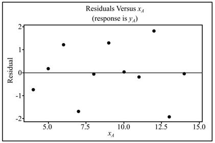
To graph: The residual versus x for each of the four datasets.
(b)
Explanation of Solution
Graph: To plot the residual versus x for each of the four datasets, Minitab is used. The steps to be followed are:
Step 1: Go to the Minitab worksheet.
Step 2: Go to Stat > Regression > Regression.
Step 3: Enter the variable
Step 4: Go to graph and select Residual versus fits.
Step 5: Click OK.
Hence, the obtained graph is
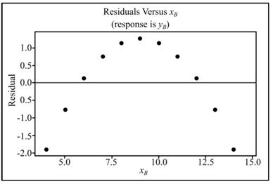
Similarly, repeat the steps for the residual plot versus x for Dataset B:
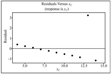
The residual plot versus x for Dataset C:
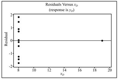
The residual plot versus x for Dataset D:
(c)
To explain: The summary for the residuals.
(c)
Answer to Problem 114E
Solution: The regression lines for datasets A and C fit the data quite well. The residual plot for dataset C shows strong
Explanation of Solution
Want to see more full solutions like this?
Chapter 2 Solutions
EBK INTRODUCTION TO THE PRACTICE OF STA


- Question 1. Your manager asks you to explain why the Black-Scholes model may be inappro- priate for pricing options in practice. Give one reason that would substantiate this claim? Question 2. We consider stock #1 and stock #2 in the model of Problem 2. Your manager asks you to pick only one of them to invest in based on the model provided. Which one do you choose and why ? Question 3. Let (St) to be an asset modeled by the Black-Scholes SDE. Let Ft be the price at time t of a European put with maturity T and strike price K. Then, the discounted option price process (ert Ft) t20 is a martingale. True or False? (Explain your answer.) Question 4. You are considering pricing an American put option using a Black-Scholes model for the underlying stock. An explicit formula for the price doesn't exist. In just a few words (no more than 2 sentences), explain how you would proceed to price it. Question 5. We model a short rate with a Ho-Lee model drt = ln(1+t) dt +2dWt. Then the interest rate…arrow_forwardIn this problem, we consider a Brownian motion (W+) t≥0. We consider a stock model (St)t>0 given (under the measure P) by d.St 0.03 St dt + 0.2 St dwt, with So 2. We assume that the interest rate is r = 0.06. The purpose of this problem is to price an option on this stock (which we name cubic put). This option is European-type, with maturity 3 months (i.e. T = 0.25 years), and payoff given by F = (8-5)+ (a) Write the Stochastic Differential Equation satisfied by (St) under the risk-neutral measure Q. (You don't need to prove it, simply give the answer.) (b) Give the price of a regular European put on (St) with maturity 3 months and strike K = 2. (c) Let X = S. Find the Stochastic Differential Equation satisfied by the process (Xt) under the measure Q. (d) Find an explicit expression for X₁ = S3 under measure Q. (e) Using the results above, find the price of the cubic put option mentioned above. (f) Is the price in (e) the same as in question (b)? (Explain why.)arrow_forwardThe managing director of a consulting group has the accompanying monthly data on total overhead costs and professional labor hours to bill to clients. Complete parts a through c. Question content area bottom Part 1 a. Develop a simple linear regression model between billable hours and overhead costs. Overhead Costsequals=212495.2212495.2plus+left parenthesis 42.4857 right parenthesis42.485742.4857times×Billable Hours (Round the constant to one decimal place as needed. Round the coefficient to four decimal places as needed. Do not include the $ symbol in your answers.) Part 2 b. Interpret the coefficients of your regression model. Specifically, what does the fixed component of the model mean to the consulting firm? Interpret the fixed term, b 0b0, if appropriate. Choose the correct answer below. A. The value of b 0b0 is the predicted billable hours for an overhead cost of 0 dollars. B. It is not appropriate to interpret b 0b0, because its value…arrow_forward
- Using the accompanying Home Market Value data and associated regression line, Market ValueMarket Valueequals=$28,416+$37.066×Square Feet, compute the errors associated with each observation using the formula e Subscript ieiequals=Upper Y Subscript iYiminus−ModifyingAbove Upper Y with caret Subscript iYi and construct a frequency distribution and histogram. LOADING... Click the icon to view the Home Market Value data. Question content area bottom Part 1 Construct a frequency distribution of the errors, e Subscript iei. (Type whole numbers.) Error Frequency minus−15 comma 00015,000less than< e Subscript iei less than or equals≤minus−10 comma 00010,000 0 minus−10 comma 00010,000less than< e Subscript iei less than or equals≤minus−50005000 5 minus−50005000less than< e Subscript iei less than or equals≤0 21 0less than< e Subscript iei less than or equals≤50005000 9…arrow_forwardThe managing director of a consulting group has the accompanying monthly data on total overhead costs and professional labor hours to bill to clients. Complete parts a through c Overhead Costs Billable Hours345000 3000385000 4000410000 5000462000 6000530000 7000545000 8000arrow_forwardUsing the accompanying Home Market Value data and associated regression line, Market ValueMarket Valueequals=$28,416plus+$37.066×Square Feet, compute the errors associated with each observation using the formula e Subscript ieiequals=Upper Y Subscript iYiminus−ModifyingAbove Upper Y with caret Subscript iYi and construct a frequency distribution and histogram. Square Feet Market Value1813 911001916 1043001842 934001814 909001836 1020002030 1085001731 877001852 960001793 893001665 884001852 1009001619 967001690 876002370 1139002373 1131001666 875002122 1161001619 946001729 863001667 871001522 833001484 798001589 814001600 871001484 825001483 787001522 877001703 942001485 820001468 881001519 882001518 885001483 765001522 844001668 909001587 810001782 912001483 812001519 1007001522 872001684 966001581 86200arrow_forward
- For a binary asymmetric channel with Py|X(0|1) = 0.1 and Py|X(1|0) = 0.2; PX(0) = 0.4 isthe probability of a bit of “0” being transmitted. X is the transmitted digit, and Y is the received digit.a. Find the values of Py(0) and Py(1).b. What is the probability that only 0s will be received for a sequence of 10 digits transmitted?c. What is the probability that 8 1s and 2 0s will be received for the same sequence of 10 digits?d. What is the probability that at least 5 0s will be received for the same sequence of 10 digits?arrow_forwardV2 360 Step down + I₁ = I2 10KVA 120V 10KVA 1₂ = 360-120 or 2nd Ratio's V₂ m 120 Ratio= 360 √2 H I2 I, + I2 120arrow_forwardQ2. [20 points] An amplitude X of a Gaussian signal x(t) has a mean value of 2 and an RMS value of √(10), i.e. square root of 10. Determine the PDF of x(t).arrow_forward
 MATLAB: An Introduction with ApplicationsStatisticsISBN:9781119256830Author:Amos GilatPublisher:John Wiley & Sons Inc
 Probability and Statistics for Engineering and th...StatisticsISBN:9781305251809Author:Jay L. DevorePublisher:Cengage Learning
 Statistics for The Behavioral Sciences (MindTap C...StatisticsISBN:9781305504912Author:Frederick J Gravetter, Larry B. WallnauPublisher:Cengage Learning
 Elementary Statistics: Picturing the World (7th E...StatisticsISBN:9780134683416Author:Ron Larson, Betsy FarberPublisher:PEARSON
 The Basic Practice of StatisticsStatisticsISBN:9781319042578Author:David S. Moore, William I. Notz, Michael A. FlignerPublisher:W. H. Freeman
 Introduction to the Practice of StatisticsStatisticsISBN:9781319013387Author:David S. Moore, George P. McCabe, Bruce A. CraigPublisher:W. H. Freeman