
To show:
The graphical representation of
Explanation of Solution
Average Cost function plays a pivotal role in establishing economies and diseconomies of scale.
Before the automation process and the assembly line production, cost of production of an automobile was exorbitant. This is shown in Panel a) of Figure 1. There were only few firms producing automobiles. Hence, their supply was limited. Average total cost of production curve AC shows the cost of Q1 of automobiles to be A1.
This cost reflects the average cost in 1901 when the technique of production to be used was limited and there were unspecialized workers. With assembly line production, division of labor was achieved. Automobile manufacturers were able to use specialized labor for specific activity. This greatly helped them in achieving economic of scale that reduced average cost of production.
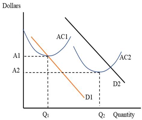
With time, there has been more use of machines that have replaced labor. This has reduced the per vehicle cost further down. This is shown by average total cost of production curve AC that shows the cost of Q2 units of automobiles to be A2 in Figure 1.
The demand curve for automobiles in 1901 was low, shown by D1 in Figure 1.People had limited financial sources to buy an automobile. Hence, they demanded fewer automobiles. With already limited supply of automobiles, the price was quite high.
By 2016, the prices have fallen because cost of production has reduced dramatically. Also, the income levels have increased for most of the consumers. This has increased their willingness to pay. Hence, the demand curve for automobiles in 2016 is higher and is shown as D2 in Figure 1.
Average Total Cost:
Average total cost is expressed as the cost incurred by the firm on the production of one unit of the output, on average. It can be measured from the total cost function when the latter is divided by the number of units produced.
Want to see more full solutions like this?
Chapter 18 Solutions
Foundations of Economics, Student Value Edition Plus MyLab Economics with eText -- Access Card Package (8th Edition)

- Q1. (Chap 1: Game Theory.) In the simultaneous games below player 1 is choosing between Top and Bottom, while player 2 is choosing between Left and Right. In each cell the first number is the payoff to player 1 and the second is the payoff to player 2. Part A: Player 1 Top Bottom Player 2 Left 25, 22 Right 27,23 26,21 28, 22 (A1) Does player 1 have a dominant strategy? (Yes/No) If your answer is yes, which one is it? (Top/Bottom) (A2) Does player 2 have a dominant strategy? (Yes/No.) If your answer is yes, which one is it? (Left/Right.) (A3) Can you solve this game by using the dominant strategy method? (Yes/No) If your answer is yes, what is the solution?arrow_forwardnot use ai pleasearrow_forwardsubject to X1 X2 Maximize dollars of interest earned = 0.07X1+0.11X2+0.19X3+0.15X4 ≤ 1,000,000 <2,500,000 X3 ≤ 1,500,000 X4 ≤ 1,800,000 X3 + XA ≥ 0.55 (X1+X2+X3+X4) X1 ≥ 0.15 (X1+X2+X3+X4) X1 + X2 X3 + XA < 5,000,000 X1, X2, X3, X4 ≥ 0arrow_forward
- Unit VI Assignment Instructions: This assignment has two parts. Answer the questions using the charts. Part 1: Firm 1 High Price Low Price High Price 8,8 0,10 Firm 2 Low Price 10,0 3,3 Question: For the above game, identify the Nash Equilibrium. Does Firm 1 have a dominant strategy? If so, what is it? Does Firm 2 have a dominant strategy? If so, what is it? Your response:arrow_forwardnot use ai please don't kdjdkdkfjnxncjcarrow_forwardAsk one question at a time. Keep questions specific and include all details. Need more help? Subject matter experts with PhDs and Masters are standing by 24/7 to answer your question.**arrow_forward
- 1b. (5 pts) Under the 1990 Farm Bill and given the initial situation of a target price and marketing loan, indicate where the market price (MP), quantity supplied (QS) and demanded (QD), government stocks (GS), and Deficiency Payments (DP) and Marketing Loan Gains (MLG), if any, would be on the graph below. If applicable, indicate the price floor (PF) on the graph. TP $ NLR So Do Q/yrarrow_forwardNow, let us assume that Brie has altruistic preferences. Her utility function is now given by: 1 UB (xA, YA, TB,YB) = (1/2) (2x+2y) + (2x+2y) What would her utility be at the endowment now? (Round off your answer to the nearest whole number.) 110arrow_forwardProblema 4 (20 puntos): Supongamos que tenemos un ingreso de $120 y enfrentamos los precios P₁ =6 y P₂ =4. Nuestra función de utilidad es: U(x1, x2) = x0.4x0.6 a) Planteen el problema de optimización y obtengan las condiciones de primer orden. b) Encuentren el consumo óptimo de x1 y x2. c) ¿Cómo cambiará nuestra elección óptima si el ingreso aumenta a $180?arrow_forward
 Managerial Economics: A Problem Solving ApproachEconomicsISBN:9781337106665Author:Luke M. Froeb, Brian T. McCann, Michael R. Ward, Mike ShorPublisher:Cengage Learning
 Microeconomics: Principles & PolicyEconomicsISBN:9781337794992Author:William J. Baumol, Alan S. Blinder, John L. SolowPublisher:Cengage Learning


 Survey of Economics (MindTap Course List)EconomicsISBN:9781305260948Author:Irvin B. TuckerPublisher:Cengage Learning