Chapter 17, Problem 41SE

The weekly demand (in cases) for a particular brand of automatic dishwasher detergent for a chain of grocery stores located in Columbus, Ohio, follows.

1. a. Construct a time series plot. What type of pattern exists in the data?
2. b. Use a three-week moving average to develop a forecast for week 11.
3. c. Use exponential smoothing with a smoothing constant of α = .2 to develop a forecast for week 11.
4. d. Which of the two methods do you prefer? Why?

To determine

Construct the time series plot.

Explain the type of pattern.

Answer to Problem 41SE

The time series plot is given below:

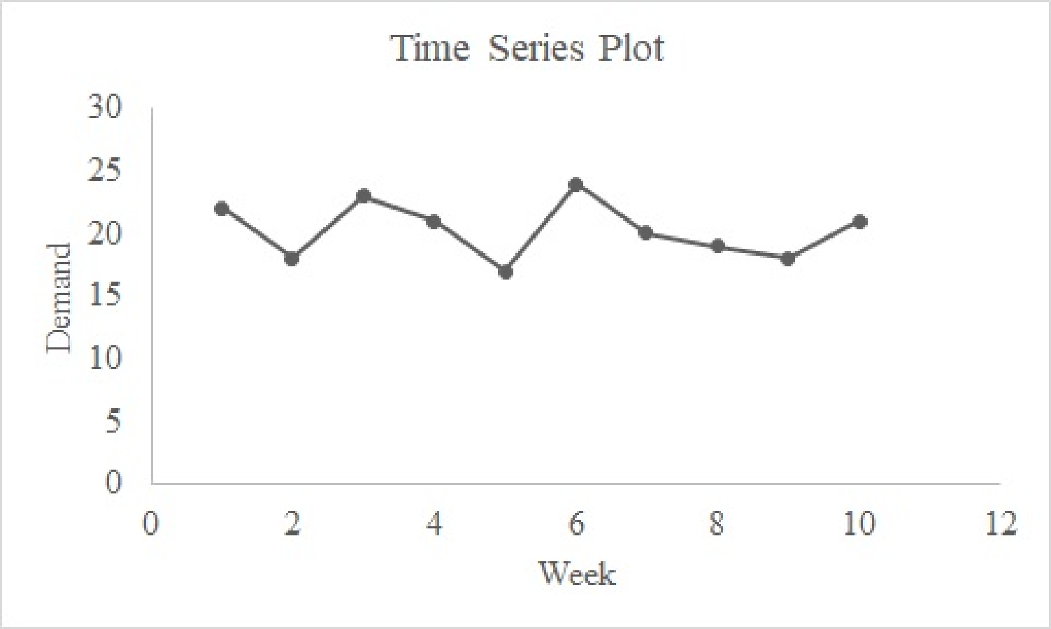
The pattern that appears in the graph is a horizontal pattern.

Explanation of Solution

Calculation:

The given data represent the weekly demand for automatic dishwasher detergent.

Software procedure:

Step-by-step software procedure to draw the time series plot using EXCEL:

• Open an EXCEL file.
• In column A, enter the data of Week, and in column B, enter the corresponding values of Demand.
• Select the data that are to be displayed.
• Click on the Insert Tab > select Scatter icon.
• Choose a Scatter with Straight Lines and Markers.
• Click on the chart > select Layout from the Chart Tools.
• Select Chart Title > Above Chart and enter Time Series Plot.
• Select Axis Title > Primary Horizontal Axis Title > Title Below Axis.
• Enter Week in the dialog box.
• Select Axis Title > Primary Vertical Axis Title > Rotated Title.
• Enter Demand in the dialog box.

From the output, the pattern that appears in the graph is a horizontal pattern.

To determine

Calculate the forecast for week 11 using three-week moving averages.

Answer to Problem 41SE

The forecast for week 11 using three-week moving averages is 19.33.

Explanation of Solution

Calculation:

The forecast for week 11 using three-week moving averages is to be obtained.

Software procedure:

Step-by-step procedure to obtain the forecasts using EXCEL:

• In column A, enter the data of Month, and in column B, enter the corresponding values of Demand.
• In Data, select Data Analysis and choose Moving Average.
• In Input Range, select Demand.
• Select Label in First Row.
• In Interval, enter 3.
• In Output Range, select C3.
• Click OK.

Output using the EXCEL software is given below:

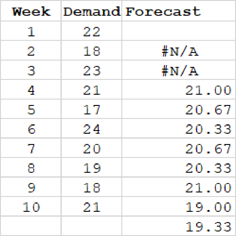
From the output, the forecast value for week 11 is 19.33.

To determine

Calculate the forecast for week 11 using the exponential smoothing with constant 0.2.

Answer to Problem 41SE

The forecast for week 11 using the exponential smoothing with constant 0.2 is 20.14.

Explanation of Solution

Calculation:

It is given that $\alpha =0.2$. Therefore, the dropping factor is 0.8 $\left(=1-0.2\right)$.

Software procedure:

Step-by-step procedure to obtain the forecasts using EXCEL:

• In column A, enter the data of Week, and in column B, enter the corresponding values of Demand.
• Select Data Analysis and choose Exponential Smoothing.
• In Input Range, select Demand.
• In Damping factor, enter 0.8.
• Select Label in First Row.
• In Output Range, select C2.
• Click OK.

Output using the EXCEL software is given below:

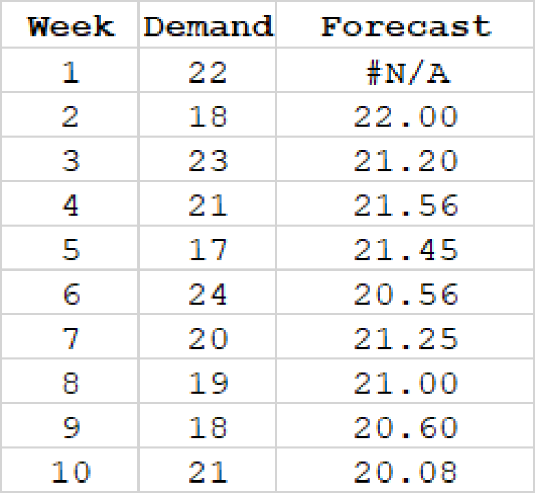
The forecast value for week 11 using exponential smoothing method is obtained as follows:

$F_{11}=\alpha Y_{10}\text{+}\left(1-\alpha \right)F_{10}$

Here, $F_{11}$ represents forecast for week 11; $Y_{10}$ represents the actual value for week 10; and $F_{10}$ represents forecast for week 10.

$\begin{array}{c}{F}_{11}=0.2\left(21\right)+\left(1-0.2\right)\left(20.08\right)\\ =4.2+16.064\\ \approx 20.26\end{array}$

Thus, the forecast value for week 11 is 20.26.

To determine

Identify the most preferable method between three-week moving averages and exponential smoothing. Explain the reason.

Answer to Problem 41SE

The three-week moving average gives the most accurate forecast because MSE for three-week moving averages is lesser when compared to the MSE for exponential smoothing.

Explanation of Solution

The formula for finding the forecast error² is as follows:

${\left(\text{Forecast error}\right)}^2={\left(\text{Actual value}-\text{Forecast}\right)}^2$

For Week 3:

The forecast error² for week 4 for 3-week moving average is obtained as follows:

$\begin{array}{c}{\left(\text{Forecast error}\right)}^2={\left(\text{Actual value}-\text{Forecast}\right)}^2\\ ={\left(260-273.33\right)}^2\\ =177.69\end{array}$

The remaining forecasts errors² for exponential smoothing averages are obtained as follows:

Week	Demand	Forecast (Ft) for 3-Week Moving Average	(Forecast Error)2	Forecast (Ft) for $\alpha =0.2$	(Forecast Error)2
1	7.35	-	-	-	-
2	7.4	-	-	22.00	16.00
3	7.55	-	-	21.20	3.24
4	7.56	21.00	0.00	21.56	0.31
5	7.6	20.67	13.44	21.45	19.78
6	7.52	20.33	13.44	20.56	11.84
7	7.52	20.67	0.44	21.25	1.55
8	7.7	20.33	1.78	21.00	3.99
9	7.62	21.00	9.00	20.60	6.75
10	7.55	19.00	4.00	20.08	0.85
Total			42.11		64.33

The MSE for 3-week moving average is obtained as follows:

$\begin{array}{c}MSE\text{=}\frac{{\text{Forecast error}}^2}{\text{Number of forecast errors}}\\ =\frac{42.11}{7}\\ =6.02\end{array}$

Thus, the value of MSE for 3-week moving average is 6.02.

The MSE for exponential smoothing averages for $\alpha =0.2$ is obtained as follows:

$\begin{array}{c}MSE\text{=}\frac{{\text{Forecast error}}^2}{\text{Number of forecast errors}}\\ =\frac{64.33}{9}\\ =7.15\end{array}$

Thus, the value of MSE for exponential smoothing averages for $\alpha =0.2$ is 7.15.

Here, it is observed that the MSE for three-week moving averages is lesser when compared to the MSE for exponential smoothing. Thus, the three-week moving average gives the most accurate forecast.