
Videos
a.
Test whether the given model is useful or not at the 0.05 level of significance.
a.
Answer to Problem 46E
There is convincing evidence that the given model is useful at the 0.05 level of significance.
Explanation of Solution
Calculation:
It is given that the variable y is absorption,
1.
The model is
2.
Null hypothesis:
That is, there is no useful relationship between y and any of the predictors.
3.
Alternative hypothesis:
That is, there is a useful relationship between y and any of the predictors.
4.
Here, the significance level is
5.
Test statistic:
Here, n is the sample size, and k is the number of variables in the model.
6.
Assumptions:
Since there is no availability of original data to check the assumptions, there is a need to assume that the variables are related to the model, and the random deviation is distributed normally with mean 0 and the fixed standard deviation.
7.
Calculation:
From the MINITAB output, the value of
The value of F-test statistic is calculated as follows:
8.
P-value:
Software procedure:
Step-by-step procedure to find the P-value using the MINITAB software:
- Choose Graph > Probability Distribution Plot choose View Probability > OK.
- From Distribution, choose ‘F’ distribution.
- Enter the Numerator df as 2 and Denominator df as 25.
- Click the Shaded Area tab.
- Choose X Value and Right Tail for the region of the curve to shade.
- Enter the X value as 334.722.
- Click OK.
Output obtained using the MINITAB software is represented as follows:
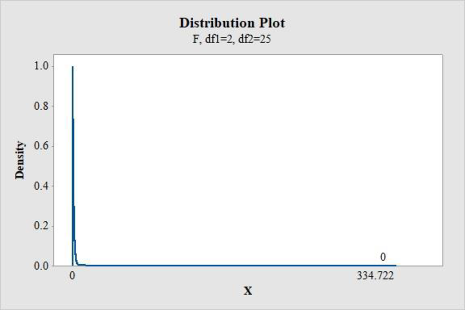
From the MINITAB output, the P-value is 0.
9.
Conclusion:
If the
Therefore, the P-value of 0 is less than the 0.05 level of significance.
Hence, reject the null hypothesis.
Thus, there is convincing evidence that the given model is useful at the 0.05 level of significance.
b.
Calculate a 95% confidence interval for
b.
Answer to Problem 46E
The 95% confidence interval for
Explanation of Solution
Calculation:
Here,
Since there is no availability of original data to check the assumptions, there is a need to assume that the variables are related to the model, and the random deviation is distributed normally with mean 0 and the fixed standard deviation.
The formula for confidence interval for
Where,
Degrees of freedom:
Software procedure:
Step-by-step procedure to find the P-value using the MINITAB software:
- Choose Graph > Probability Distribution Plot choose View Probability > OK.
- From Distribution, choose ‘t’ distribution.
- Enter the Degrees of freedom as 25.
- Click the Shaded Area tab.
- Choose Probability and Both for the region of the curve to shade.
- Enter the Probability value as 0.05.
- Click OK.
Output obtained using the MINITAB software is represented as follows:
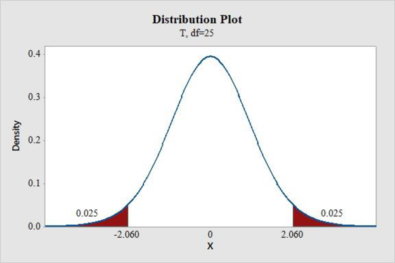
From the MINITAB output, the critical value is 2.060.
From the given MINITAB output, the value of
The confidence interval for mean change in exam score is calculated as follows:
Thus, the 95% confidence interval for
There is 95% confident that the average increase in y is associated with 1-unit increase in starch damage that is between 0.298 and 0.373, when the other predictors are fixed.
c.
- i. Test the hypothesis
H 0 : β 1 = 0 H a : β 1 ≠ 0
- ii. Test the hypothesis
H 0 : β 2 = 0 H a : β 2 ≠ 0
c.
Answer to Problem 46E
It can be concluded that the quadratic term should not be eliminated from the model and simple linear model should not be sufficient.
Explanation of Solution
Calculation:
i.
1.
The predictor
2.
Null hypothesis:
3.
Alternative hypothesis:
4.
Here, the common significance levels are
5.
Test statistic:
Here,
6.
Assumptions:
The random deviations from the values by the population regression equation are distributed normally with mean 0 and fixed standard deviation.
7.
Calculation:
From the MINITAB output, the t test statistic value of
8.
P-value:
From the MINITAB output, the P-value for
9.
Conclusion:
If the
Therefore, the P-value of 0 is less than any common levels of significance, such as 0.05, 0.01, and 0.10.
Hence, reject the null hypothesis.
Thus, there is convincing evidence that the flour protein variable is important and it is
ii.
1.
The predictor
2.
Null hypothesis:
3.
Alternative hypothesis:
4.
Here, the common significance levels are
5.
Test statistic:
Here,
6.
Assumptions:
The random deviations from the values by the population regression equation are distributed normally with mean 0 and fixed standard deviation.
7.
Calculation:
From the MINITAB output, the t test statistic value of
8.
P-value:
From the MINITAB output, the P-value for
9.
Conclusion:
If the
Therefore, the P-value of 0 is less than any common levels of significance, such as 0.05, 0.01, and 0.10.
Hence, reject the null hypothesis.
Thus, there is convincing evidence that the starch damage variable is important and it is
d.
Explain whether both the independent variables are important or not.
d.
Explanation of Solution
From the results of Part (c), there is evidence that the variables of flour protein and starch damage are important.
e.
Calculate a 90% confidence interval and interpret it.
e.
Answer to Problem 46E
The 90% confidence interval is
Explanation of Solution
Calculation:
It is given that the value of
Assume that the exam score is associated with the predictors according to the model. The random deviations from the values by the population regression equation are distributed normally with mean 0 and fixed standard deviation.
The formula for prediction interval for mean y value is as follows:
The value of
Degrees of freedom:
Software procedure:
Step-by-step procedure to find the P-value using the MINITAB software:
- Choose Graph > Probability Distribution Plot choose View Probability > OK.
- From Distribution, choose ‘t’ distribution.
- Enter the Degrees of freedom as 25.
- Click the Shaded Area tab.
- Choose Probability and Both for the region of the curve to shade.
- Enter the Probability value as 0.10.
- Click OK.
Output obtained using the MINITAB software is represented as follows:
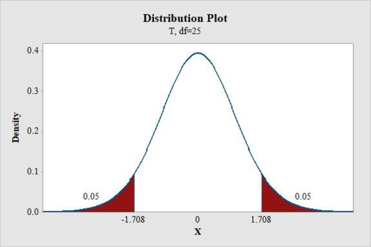
From the MINITAB output, the critical value is 1.708.
The prediction interval for mean y value is calculated as follows:
Thus, the 90% confidence interval is
There is 90% confident that the mean water absorption for wheat with 11.7 flour protein and 57 starch damage is between 54.5084 and 56.2916.
f.
Predict the water absorption for the shipment by 90% interval.
f.
Answer to Problem 46E
The water absorption values for the particular shipment are between 53.3297 and 57.4703 by 90% prediction interval.
Explanation of Solution
Calculation:
It is given that the value of
Assume that the exam score is associated with the predictors according to the model. The random deviations from the values by the population regression equation are distributed normally with mean 0 and fixed standard deviation.
The formula for prediction interval for mean y value is as follows:
From the given MINITAB output, the standard deviation is 1.094.
From Part e., the value of
From the MINITAB output in Part e., the critical value is 1.708.
The prediction interval for water absorption for shipment is calculated as follows:
Thus, the 90% prediction interval is
By prediction at 90% interval, the water absorption values for the particular shipment are between 53.3297 and 57.4703.
Want to see more full solutions like this?
Chapter 14 Solutions
Introduction To Statistics And Data Analysis


- Q.2.4 There are twelve (12) teams participating in a pub quiz. What is the probability of correctly predicting the top three teams at the end of the competition, in the correct order? Give your final answer as a fraction in its simplest form.arrow_forwardThe table below indicates the number of years of experience of a sample of employees who work on a particular production line and the corresponding number of units of a good that each employee produced last month. Years of Experience (x) Number of Goods (y) 11 63 5 57 1 48 4 54 5 45 3 51 Q.1.1 By completing the table below and then applying the relevant formulae, determine the line of best fit for this bivariate data set. Do NOT change the units for the variables. X y X2 xy Ex= Ey= EX2 EXY= Q.1.2 Estimate the number of units of the good that would have been produced last month by an employee with 8 years of experience. Q.1.3 Using your calculator, determine the coefficient of correlation for the data set. Interpret your answer. Q.1.4 Compute the coefficient of determination for the data set. Interpret your answer.arrow_forwardCan you answer this question for mearrow_forward
- Techniques QUAT6221 2025 PT B... TM Tabudi Maphoru Activities Assessments Class Progress lIE Library • Help v The table below shows the prices (R) and quantities (kg) of rice, meat and potatoes items bought during 2013 and 2014: 2013 2014 P1Qo PoQo Q1Po P1Q1 Price Ро Quantity Qo Price P1 Quantity Q1 Rice 7 80 6 70 480 560 490 420 Meat 30 50 35 60 1 750 1 500 1 800 2 100 Potatoes 3 100 3 100 300 300 300 300 TOTAL 40 230 44 230 2 530 2 360 2 590 2 820 Instructions: 1 Corall dawn to tha bottom of thir ceraan urina se se tha haca nariad in archerca antarand cubmit Q Search ENG US 口X 2025/05arrow_forwardThe table below indicates the number of years of experience of a sample of employees who work on a particular production line and the corresponding number of units of a good that each employee produced last month. Years of Experience (x) Number of Goods (y) 11 63 5 57 1 48 4 54 45 3 51 Q.1.1 By completing the table below and then applying the relevant formulae, determine the line of best fit for this bivariate data set. Do NOT change the units for the variables. X y X2 xy Ex= Ey= EX2 EXY= Q.1.2 Estimate the number of units of the good that would have been produced last month by an employee with 8 years of experience. Q.1.3 Using your calculator, determine the coefficient of correlation for the data set. Interpret your answer. Q.1.4 Compute the coefficient of determination for the data set. Interpret your answer.arrow_forwardQ.3.2 A sample of consumers was asked to name their favourite fruit. The results regarding the popularity of the different fruits are given in the following table. Type of Fruit Number of Consumers Banana 25 Apple 20 Orange 5 TOTAL 50 Draw a bar chart to graphically illustrate the results given in the table.arrow_forward
- Q.2.3 The probability that a randomly selected employee of Company Z is female is 0.75. The probability that an employee of the same company works in the Production department, given that the employee is female, is 0.25. What is the probability that a randomly selected employee of the company will be female and will work in the Production department? Q.2.4 There are twelve (12) teams participating in a pub quiz. What is the probability of correctly predicting the top three teams at the end of the competition, in the correct order? Give your final answer as a fraction in its simplest form.arrow_forwardQ.2.1 A bag contains 13 red and 9 green marbles. You are asked to select two (2) marbles from the bag. The first marble selected will not be placed back into the bag. Q.2.1.1 Construct a probability tree to indicate the various possible outcomes and their probabilities (as fractions). Q.2.1.2 What is the probability that the two selected marbles will be the same colour? Q.2.2 The following contingency table gives the results of a sample survey of South African male and female respondents with regard to their preferred brand of sports watch: PREFERRED BRAND OF SPORTS WATCH Samsung Apple Garmin TOTAL No. of Females 30 100 40 170 No. of Males 75 125 80 280 TOTAL 105 225 120 450 Q.2.2.1 What is the probability of randomly selecting a respondent from the sample who prefers Garmin? Q.2.2.2 What is the probability of randomly selecting a respondent from the sample who is not female? Q.2.2.3 What is the probability of randomly…arrow_forwardTest the claim that a student's pulse rate is different when taking a quiz than attending a regular class. The mean pulse rate difference is 2.7 with 10 students. Use a significance level of 0.005. Pulse rate difference(Quiz - Lecture) 2 -1 5 -8 1 20 15 -4 9 -12arrow_forward
- The following ordered data list shows the data speeds for cell phones used by a telephone company at an airport: A. Calculate the Measures of Central Tendency from the ungrouped data list. B. Group the data in an appropriate frequency table. C. Calculate the Measures of Central Tendency using the table in point B. D. Are there differences in the measurements obtained in A and C? Why (give at least one justified reason)? I leave the answers to A and B to resolve the remaining two. 0.8 1.4 1.8 1.9 3.2 3.6 4.5 4.5 4.6 6.2 6.5 7.7 7.9 9.9 10.2 10.3 10.9 11.1 11.1 11.6 11.8 12.0 13.1 13.5 13.7 14.1 14.2 14.7 15.0 15.1 15.5 15.8 16.0 17.5 18.2 20.2 21.1 21.5 22.2 22.4 23.1 24.5 25.7 28.5 34.6 38.5 43.0 55.6 71.3 77.8 A. Measures of Central Tendency We are to calculate: Mean, Median, Mode The data (already ordered) is: 0.8, 1.4, 1.8, 1.9, 3.2, 3.6, 4.5, 4.5, 4.6, 6.2, 6.5, 7.7, 7.9, 9.9, 10.2, 10.3, 10.9, 11.1, 11.1, 11.6, 11.8, 12.0, 13.1, 13.5, 13.7, 14.1, 14.2, 14.7, 15.0, 15.1, 15.5,…arrow_forwardPEER REPLY 1: Choose a classmate's Main Post. 1. Indicate a range of values for the independent variable (x) that is reasonable based on the data provided. 2. Explain what the predicted range of dependent values should be based on the range of independent values.arrow_forwardIn a company with 80 employees, 60 earn $10.00 per hour and 20 earn $13.00 per hour. Is this average hourly wage considered representative?arrow_forward
 MATLAB: An Introduction with ApplicationsStatisticsISBN:9781119256830Author:Amos GilatPublisher:John Wiley & Sons Inc
 Probability and Statistics for Engineering and th...StatisticsISBN:9781305251809Author:Jay L. DevorePublisher:Cengage Learning
 Statistics for The Behavioral Sciences (MindTap C...StatisticsISBN:9781305504912Author:Frederick J Gravetter, Larry B. WallnauPublisher:Cengage Learning
 Elementary Statistics: Picturing the World (7th E...StatisticsISBN:9780134683416Author:Ron Larson, Betsy FarberPublisher:PEARSON
 The Basic Practice of StatisticsStatisticsISBN:9781319042578Author:David S. Moore, William I. Notz, Michael A. FlignerPublisher:W. H. Freeman
 Introduction to the Practice of StatisticsStatisticsISBN:9781319013387Author:David S. Moore, George P. McCabe, Bruce A. CraigPublisher:W. H. Freeman