
Concept explainers
Videos
Have you ever wondered whether soccer players suffer adverse effects from hitting “headers”? The authors of the article “No Evidence of Impaired Neurocognitive Performance in Collegiate Soccer Players” (Amer. J. of Sports Med., 2002: 157–162) investigated this issue from several perspectives.
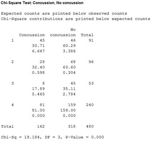
a. The paper reported that 45 of the 91 soccer players in their sample had suffered at least one concussion, 28 of 96 nonsoccer athletes had suffered at least one concussion, and only 8 of 53 student controls had suffered at least one concussion. Analyze this data and draw appropriate conclusions.
b. For the soccer players, the sample
c. Here is summary information on scores on a controlled oral word-association test for the soccer and nonsoccer athletes:
Analyze this data and draw appropriate conclusions.
d. Considering the number of prior nonsoccer concussions, the values of mean 6 sd for the three groups were .30 ± .67, .49 ± .87, and .19 ± .48. Analyze this data and draw appropriate conclusions.
a.
Analyze the given data and draw conclusions.
Answer to Problem 47SE
There is sufficient evidence to conclude that there is a difference in the proportion of concussion with respect to three groups.
Explanation of Solution
Given info:
The report says that 45 out of 91 soccer players had suffered at least one concussion, 28 of 96 non-soccer athletes suffered at least one concussion and 8 of 53 students had at least one concussion.
Calculation:
From the given data the following can be observed,
| Group | Concussion | No concussion | Total |
| Soccer | 45 | 46 | 91 |
| Non soccer | 28 | 68 | 96 |
| student | 8 | 45 | 53 |
| Total | 81 | 159 | 240 |
The claim is to test whether there is any homogeneity among the proportion of concussions with respect to the three groups. If the claim is rejected, then there is no homogeneity among the proportion of concussions with respect to the three groups.
Null hypothesis:
That is, the proportion of concussions is homogenous with respect to the three groups.
Alternative hypothesis:
Test statistic:
Software procedure:
Step-by-step procedure to find the chi-square test statistic using MINITAB is given below:
- Choose Stat > Tables > Chi-Square Test (Two-Way Table in Worksheet).
- In Columns containing the table, enter the columns of Concussion and Nonconcussion.
- Click OK.
Output obtained from MINITAB is given below:
Decision rule:
If
If
Conclusion:
The P-value is 0.000 and the least level of significance is 0.001.
The P-value is lesser than the level of significance.
That is,
Thus, the null hypothesis isrejected.
Hence, there is sufficient evidence to conclude that there is a difference in the proportion of concussion with respect to three groups.
b.
Interpret the given results.
Answer to Problem 47SE
There is no sufficient evidence to conclude that there exists a negative correlation or association in the population at 1% level of significance.
Explanation of Solution
Given info:
The sample correlation coefficient for the soccer players group is calculated by using the soccer exposure x and the score on an immediate memory recall test y and it is –0.220.
Calculation:
Testing the significance of correlation:
Null hypothesis:
That is, there is no correlation between x and y.
Alternative hypothesis:
That is, there is a negative correlation between x and y.
Test statistic:
Where,
r represents the correlation coefficient value.
n represents the total sample size.
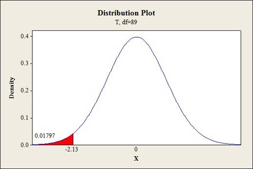
Substitute r as –0.220 and n as 91.
Thus, the test statistic is –2.13.
P-value:
Software procedure:
Step-by-step procedure to obtain the P-value is given below:
- Click on Graph, select View Probability and click OK.
- Select t, enter 89 in degrees of freedom..
- Under Shaded Area Tab select X value under Define Shaded Area By and select left tail.
- Choose X value as –2.13.
- Click OK.
Output obtained from MINITAB is given below:
Conclusion:
The P-valueis 0.018 and the level of significance is 0.01.
The P-valueis lesser than the level of significance.
That is,
Thus, the null hypothesis is not rejected.
Hence, there is no sufficient evidence to conclude that there exists a negative correlation or association in the population at 1% level of significance.
c.
Analyze the given data and draw conclusions.
Answer to Problem 47SE
There is sufficient evidence to conclude that the average scores of two groups are the same.
Explanation of Solution
Given info:
An oral test was conducted for soccer and non-soccer athletes. The summary statistics are given below:
Calculation:
Testing the hypothesis:
Null hypothesis:
That is, the average test score is same for the two groups.
Alternative hypothesis:
That is, the average test score is not the same for the two groups.
Test statistic:
Software procedure:
Step-by-step procedure to obtain the test statistic using MINITAB is given below:
- Choose Stat > Basic Statistics > 2-Sample t.
- Choose Summarized data.
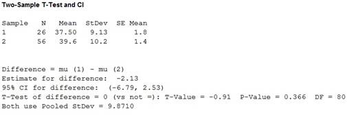
- In first, enter Sample size as 26, Mean as 37.50, Standard deviation as 9.13.
- In second, enter Sample size as56, Mean as 39.63, Standard deviation as 10.19.
- Select Assume equal variances.
- Choose Options.
- In Confidence level, enter 95.
- Choose not equal in Alternative.
- Click OK.
Output obtained from MINITAB is given below:
Conclusion:
The P-value is 0.366 and the level of significance is 0.10.
The P-value is greater than the level of significance.
That is,
Thus, the null hypothesis is not rejected.
Hence, there is sufficient evidence to conclude that the average scores of two groups are the same.
d.
Analyze the given data and draw conclusions.
Answer to Problem 47SE
There is sufficient evidence to conclude that there is a difference in the average number of prior non-soccer concussion between the three groups.
Explanation of Solution
Given info:
The mean plus or standard deviation for the three groups with respect to the number of prior non-soccer concussions are
Calculation:
Testing the hypothesis:
Null hypothesis:
That is, there is no difference in the average number of prior non-soccer concussion between the three groups.
Alternative hypothesis:
That is, there is a difference in the average number of prior non-soccer concussion between the three groups.
Test statistic:
Where,
MSE represents the mean sum of squares due to error.
Sum of squares with respect to the three groups is calculated as follows:
Where,
Mean sum of squares due to treatment:
Sum of squares due to error:
Mean sum of squares due to error:
Thus, the F-statistic is calculated as follows:
Critical value:
Software procedure:
Step-by-step procedure to obtain the P-value is given below:
- Click on Graph, select View Probability and click OK.
- Select F, enter 2 in numerator df and 236 in denominator df.
- Under Shaded Area Tab select X value under Define Shaded Area By and select right tail.
- Choose Probability as 0.05.
- Click OK.
Output obtained from MINITAB is given below:
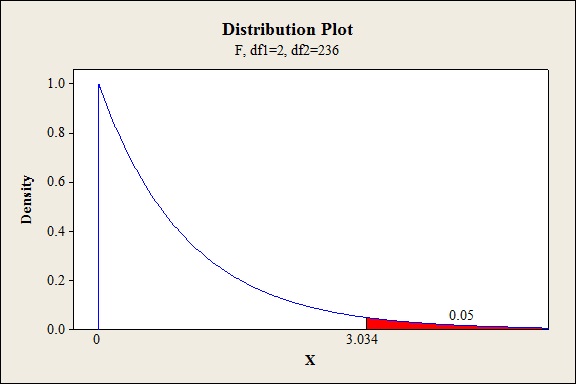
Thus, the critical value is 3.034.
Conclusion:
The test statisticis 3.319and the critical value is 3.034.
The test statisticis lesser than the critical value.
That is,
Thus, the null hypothesis is rejected.
Hence, there is sufficient evidence to conclude that there is a difference in the average number of prior non-soccer concussion between the three groups.
Want to see more full solutions like this?
Chapter 14 Solutions
Probability and Statistics for Engineering and the Sciences STAT 400 - University Of Maryland


- You find out that the dietary scale you use each day is off by a factor of 2 ounces (over — at least that’s what you say!). The margin of error for your scale was plus or minus 0.5 ounces before you found this out. What’s the margin of error now?arrow_forwardSuppose that Sue and Bill each make a confidence interval out of the same data set, but Sue wants a confidence level of 80 percent compared to Bill’s 90 percent. How do their margins of error compare?arrow_forwardSuppose that you conduct a study twice, and the second time you use four times as many people as you did the first time. How does the change affect your margin of error? (Assume the other components remain constant.)arrow_forward
- Out of a sample of 200 babysitters, 70 percent are girls, and 30 percent are guys. What’s the margin of error for the percentage of female babysitters? Assume 95 percent confidence.What’s the margin of error for the percentage of male babysitters? Assume 95 percent confidence.arrow_forwardYou sample 100 fish in Pond A at the fish hatchery and find that they average 5.5 inches with a standard deviation of 1 inch. Your sample of 100 fish from Pond B has the same mean, but the standard deviation is 2 inches. How do the margins of error compare? (Assume the confidence levels are the same.)arrow_forwardA survey of 1,000 dental patients produces 450 people who floss their teeth adequately. What’s the margin of error for this result? Assume 90 percent confidence.arrow_forward
- The annual aggregate claim amount of an insurer follows a compound Poisson distribution with parameter 1,000. Individual claim amounts follow a Gamma distribution with shape parameter a = 750 and rate parameter λ = 0.25. 1. Generate 20,000 simulated aggregate claim values for the insurer, using a random number generator seed of 955.Display the first five simulated claim values in your answer script using the R function head(). 2. Plot the empirical density function of the simulated aggregate claim values from Question 1, setting the x-axis range from 2,600,000 to 3,300,000 and the y-axis range from 0 to 0.0000045. 3. Suggest a suitable distribution, including its parameters, that approximates the simulated aggregate claim values from Question 1. 4. Generate 20,000 values from your suggested distribution in Question 3 using a random number generator seed of 955. Use the R function head() to display the first five generated values in your answer script. 5. Plot the empirical density…arrow_forwardFind binomial probability if: x = 8, n = 10, p = 0.7 x= 3, n=5, p = 0.3 x = 4, n=7, p = 0.6 Quality Control: A factory produces light bulbs with a 2% defect rate. If a random sample of 20 bulbs is tested, what is the probability that exactly 2 bulbs are defective? (hint: p=2% or 0.02; x =2, n=20; use the same logic for the following problems) Marketing Campaign: A marketing company sends out 1,000 promotional emails. The probability of any email being opened is 0.15. What is the probability that exactly 150 emails will be opened? (hint: total emails or n=1000, x =150) Customer Satisfaction: A survey shows that 70% of customers are satisfied with a new product. Out of 10 randomly selected customers, what is the probability that at least 8 are satisfied? (hint: One of the keyword in this question is “at least 8”, it is not “exactly 8”, the correct formula for this should be = 1- (binom.dist(7, 10, 0.7, TRUE)). The part in the princess will give you the probability of seven and less than…arrow_forwardplease answer these questionsarrow_forward
- Selon une économiste d’une société financière, les dépenses moyennes pour « meubles et appareils de maison » ont été moins importantes pour les ménages de la région de Montréal, que celles de la région de Québec. Un échantillon aléatoire de 14 ménages pour la région de Montréal et de 16 ménages pour la région Québec est tiré et donne les données suivantes, en ce qui a trait aux dépenses pour ce secteur d’activité économique. On suppose que les données de chaque population sont distribuées selon une loi normale. Nous sommes intéressé à connaitre si les variances des populations sont égales.a) Faites le test d’hypothèse sur deux variances approprié au seuil de signification de 1 %. Inclure les informations suivantes : i. Hypothèse / Identification des populationsii. Valeur(s) critique(s) de Fiii. Règle de décisioniv. Valeur du rapport Fv. Décision et conclusion b) A partir des résultats obtenus en a), est-ce que l’hypothèse d’égalité des variances pour cette…arrow_forwardAccording to an economist from a financial company, the average expenditures on "furniture and household appliances" have been lower for households in the Montreal area than those in the Quebec region. A random sample of 14 households from the Montreal region and 16 households from the Quebec region was taken, providing the following data regarding expenditures in this economic sector. It is assumed that the data from each population are distributed normally. We are interested in knowing if the variances of the populations are equal. a) Perform the appropriate hypothesis test on two variances at a significance level of 1%. Include the following information: i. Hypothesis / Identification of populations ii. Critical F-value(s) iii. Decision rule iv. F-ratio value v. Decision and conclusion b) Based on the results obtained in a), is the hypothesis of equal variances for this socio-economic characteristic measured in these two populations upheld? c) Based on the results obtained in a),…arrow_forwardA major company in the Montreal area, offering a range of engineering services from project preparation to construction execution, and industrial project management, wants to ensure that the individuals who are responsible for project cost estimation and bid preparation demonstrate a certain uniformity in their estimates. The head of civil engineering and municipal services decided to structure an experimental plan to detect if there could be significant differences in project evaluation. Seven projects were selected, each of which had to be evaluated by each of the two estimators, with the order of the projects submitted being random. The obtained estimates are presented in the table below. a) Complete the table above by calculating: i. The differences (A-B) ii. The sum of the differences iii. The mean of the differences iv. The standard deviation of the differences b) What is the value of the t-statistic? c) What is the critical t-value for this test at a significance level of 1%?…arrow_forward
 Glencoe Algebra 1, Student Edition, 9780079039897...AlgebraISBN:9780079039897Author:CarterPublisher:McGraw Hill
 Holt Mcdougal Larson Pre-algebra: Student Edition...AlgebraISBN:9780547587776Author:HOLT MCDOUGALPublisher:HOLT MCDOUGAL
 College Algebra (MindTap Course List)AlgebraISBN:9781305652231Author:R. David Gustafson, Jeff HughesPublisher:Cengage Learning
 Big Ideas Math A Bridge To Success Algebra 1: Stu...AlgebraISBN:9781680331141Author:HOUGHTON MIFFLIN HARCOURTPublisher:Houghton Mifflin Harcourt