Videos
a.
Test whether the data suggests a linear relationship between specific gravity and at least one of the predictors at 1% level of significance.
a.
Answer to Problem 56E
There is sufficient evidence to conclude that the there is a use of linear relationship between specific gravity and at least one of the five predictors number of fibers in springwood, number of fibers in summerwood, percentage of springwood, light absorption in springwood and light absorption in summerwood at 1% level of significance.
Explanation of Solution
Given info:
A sample of 20 mature woods were taken and the number of fibers in springwood, number of fibers in summerwood, percentage of springwood, light absorption in springwood and light absorption in summerwood were noted .
The coefficient of determination
Calculation:
The test hypotheses are given below:
Null hypothesis:
That is, there is no use of linear relationship between specific gravity and the five predictors.
Alternative hypothesis:
That is, there is a use of linear relationship between specific gravity and at least one of the five predictors.
Test statistic:
Substitute
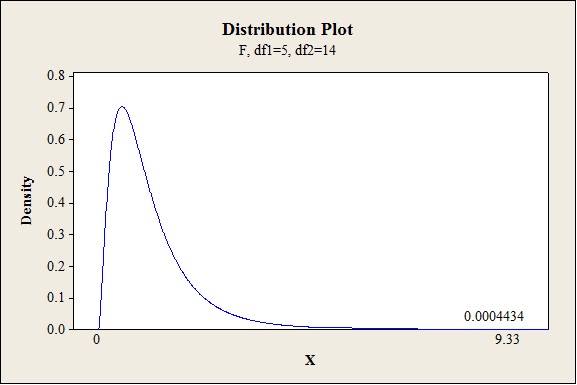
P-value:
Software procedure:
- Click on Graph, select View Probability and click OK.
- Select F, enter 5 in numerator df and 14 in denominator df.
- Under Shaded Area Tab select X value under Define Shaded Area By and select Right tail.
- Choose X value as 9.33.
- Click OK.
Output obtained from MINITAB is given below:
Conclusion:
The P-value is 0.000 and the level of significance is 0.01.
The P-value is lesser than the level of significance.
That is
Thus, the null hypothesis is rejected.
Hence, there is sufficient evidence to conclude that there is ause of linear relationship between specific gravity and at least one of the five predictors at 1% level of significance.
b.
Calculate the adjusted
b.
Answer to Problem 56E
The adjusted
The adjusted
Explanation of Solution
Given info:
The
Calculation:
Adjusted
Adjusted
Substitute n as 20,k as 5,
Thus, the adjusted
Adjusted
Substitute n as 20, k as 4,
Thus, the adjusted
c.
Identify whether the data suggests that variables
Test the hypothesis to see whether the variables
c.
Answer to Problem 56E
Yes, the data suggests that variables
There issufficient evidence to conclude the variables
Explanation of Solution
Given info:
The
Calculation:
After dropping the three variables
The test hypotheses are given below:
Null hypothesis:
That is, there is no use of linear relationship betweenspecific gravity and at least one of the predictors, percentage of springwood and light absorption in summerwood.
Alternative hypothesis:
That is, there is use of linear relationship between specific gravity and at least one of the predictors, percentage of springwood and light absorption in summerwood.
From the
Similarly, the sum of squares due to error for the reduced model
Test statistic:
Where,
n represents the total number of observations.
k represents the number of predictors on the full model.
l represents the number of predictors on the reduced model.
Substitute 0.004542for
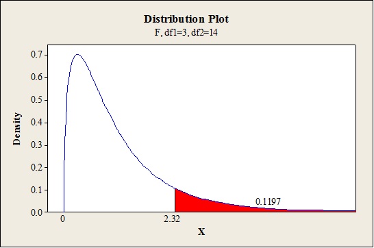
Critical value:
Software procedure:
- Click on Graph, select View Probability and click OK.
- Select F, enter 3 in numerator df and 14 in denominator df.
- Under Shaded Area Tab select Probability under Define Shaded Area By and select Right tail.
- Choose X Value as 2.32.
- Click OK.
Output obtained from MINITAB is given below:
Conclusion:
The P-value is 0.1197 and the level of significance is 0.05.
The P-value is lesser than the level of significance.
That is,
Thus, the null hypothesis is not rejected.
Hence, there is no sufficient evidence to conclude that there is a use of linear relationship betweenspecific gravity and at least one of the predictor percentage of springwood and light absorption in summerwood at 5% level of significance.
Thus, the variables
d.
Predict the value of specific gravity when the percentage of springwood is 50 and percentage of light absorption in summerwood is 90.
d.
Answer to Problem 56E
The estimated value for specific gravity when the percentage of springwood is 50 and percentage of light absorption in summerwood is 90 is 0.5386.
Explanation of Solution
Given info:
The mean and standard deviation for the variable
The estimated regression equation after standardization is
Calculation:
The standardized values
Where,
The standardized value when mean and standard deviation for the variable
Thus, the value of
The standardized value when the mean and standard deviation for the variable
Thus, the value of
The estimated value for specific gravity is,
Thus, the estimated value for specific gravity when the percentage of springwood is 50 and percentage of light absorption in summerwood is 90 is 0.5386.
e.
Find the 95% confidence interval for the estimated coefficient of
e.
Answer to Problem 56E
The 95% confidence interval for the estimated coefficient of
Explanation of Solution
Calculation:
95% confidence interval:
The confidence interval is calculated using the formula:
Where,
n is the total number of observations.
k is the total number of predictors in the model.
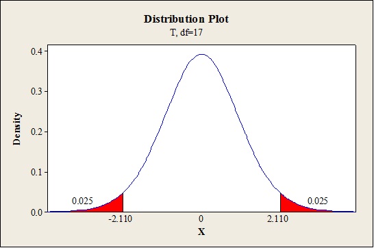
Critical value:
Software procedure:
Step-by-step procedure to find the critical value is given below:
- Click on Graph, select View Probability and click OK.
- Select t, enter 17 as Degrees of freedom, in Shaded Area Tab select Probability under Define Shaded Area By and choose Both tails.
- Enter Probability value as 0.05.
- Click OK.
Output obtained from MINITAB is given below:
The 95% confidence interval is given below:
Thus, the 95% confidence interval for the estimated coefficient of
f.
Find the estimated coefficient and estimated standard deviation of
f.
Answer to Problem 56E
The estimated coefficient of
The estimated standard deviation of
Explanation of Solution
Given info:
Use the information given in part (d) and (e).
Calculation:
The estimated regression equation for standardized model is,
The estimated coefficient of
Thus, the estimated coefficient of
The estimate for
The estimated standard deviation for
Thus, the estimated standard deviation of
g.
Find the 95% prediction interval for the specific gravity when the percentage of spring wood is 50.5 and percentage of light absorption in summerwood is 88.9.
g.
Answer to Problem 56E
The 95% prediction interval for the specific gravity when the percentage of spring wood is 50.5 and percentage of light absorption in summerwood is 88.9 is(0.489, 0.575).
Explanation of Solution
Given info:
The estimated standard deviation for the model with two predictors is 0.02001. The estimated standard deviation for the predicated value when the coefficients
Calculation:
The predicted value for the specific gravity when the percentage of spring wood is 50.5 and percentage of light absorption in summerwood is 88.9 is calculated as follows:
Thus, the predicted value for the specific gravity when the percentage of spring wood is 50.5 and percentage of light absorption in summerwood is 88.9 is 0.532.
95% prediction interval:
The confidence interval is calculated using the formula:
Where,
n is the total number of observations.
k is the total number of predictors in the model.
s is the overall standard deviation obtained after fitting the model.
Critical value:
Software procedure:
Step-by-step procedure to find the critical value is given below:
- Click on Graph, select View Probability and click OK.
- Select t, enter 17 as Degrees of freedom, in Shaded Area Tab select Probability under Define Shaded Area By and choose Both tails.
- Enter Probability value as 0.05.
- Click OK.
Output obtained from MINITAB is given below:
The 95% prediction interval is given below:
Thus, the 95% prediction interval for the specific gravity when the percentage of spring wood is 50.5 and percentage of light absorption in summerwood is 88.9 is (0.489,0.575).
Want to see more full solutions like this?
Chapter 13 Solutions
Probability and Statistics for Engineering and the Sciences STAT 400 - University Of Maryland


- Pls help asaparrow_forwardSolve the following LP problem using the Extreme Point Theorem: Subject to: Maximize Z-6+4y 2+y≤8 2x + y ≤10 2,y20 Solve it using the graphical method. Guidelines for preparation for the teacher's questions: Understand the basics of Linear Programming (LP) 1. Know how to formulate an LP model. 2. Be able to identify decision variables, objective functions, and constraints. Be comfortable with graphical solutions 3. Know how to plot feasible regions and find extreme points. 4. Understand how constraints affect the solution space. Understand the Extreme Point Theorem 5. Know why solutions always occur at extreme points. 6. Be able to explain how optimization changes with different constraints. Think about real-world implications 7. Consider how removing or modifying constraints affects the solution. 8. Be prepared to explain why LP problems are used in business, economics, and operations research.arrow_forwardged the variance for group 1) Different groups of male stalk-eyed flies were raised on different diets: a high nutrient corn diet vs. a low nutrient cotton wool diet. Investigators wanted to see if diet quality influenced eye-stalk length. They obtained the following data: d Diet Sample Mean Eye-stalk Length Variance in Eye-stalk d size, n (mm) Length (mm²) Corn (group 1) 21 2.05 0.0558 Cotton (group 2) 24 1.54 0.0812 =205-1.54-05T a) Construct a 95% confidence interval for the difference in mean eye-stalk length between the two diets (e.g., use group 1 - group 2).arrow_forward
- An article in Business Week discussed the large spread between the federal funds rate and the average credit card rate. The table below is a frequency distribution of the credit card rate charged by the top 100 issuers. Credit Card Rates Credit Card Rate Frequency 18% -23% 19 17% -17.9% 16 16% -16.9% 31 15% -15.9% 26 14% -14.9% Copy Data 8 Step 1 of 2: Calculate the average credit card rate charged by the top 100 issuers based on the frequency distribution. Round your answer to two decimal places.arrow_forwardPlease could you check my answersarrow_forwardLet Y₁, Y2,, Yy be random variables from an Exponential distribution with unknown mean 0. Let Ô be the maximum likelihood estimates for 0. The probability density function of y; is given by P(Yi; 0) = 0, yi≥ 0. The maximum likelihood estimate is given as follows: Select one: = n Σ19 1 Σ19 n-1 Σ19: n² Σ1arrow_forward
- Please could you help me answer parts d and e. Thanksarrow_forwardWhen fitting the model E[Y] = Bo+B1x1,i + B2x2; to a set of n = 25 observations, the following results were obtained using the general linear model notation: and 25 219 10232 551 XTX = 219 10232 3055 133899 133899 6725688, XTY 7361 337051 (XX)-- 0.1132 -0.0044 -0.00008 -0.0044 0.0027 -0.00004 -0.00008 -0.00004 0.00000129, Construct a multiple linear regression model Yin terms of the explanatory variables 1,i, x2,i- a) What is the value of the least squares estimate of the regression coefficient for 1,+? Give your answer correct to 3 decimal places. B1 b) Given that SSR = 5550, and SST=5784. Calculate the value of the MSg correct to 2 decimal places. c) What is the F statistics for this model correct to 2 decimal places?arrow_forwardCalculate the sample mean and sample variance for the following frequency distribution of heart rates for a sample of American adults. If necessary, round to one more decimal place than the largest number of decimal places given in the data. Heart Rates in Beats per Minute Class Frequency 51-58 5 59-66 8 67-74 9 75-82 7 83-90 8arrow_forward
- can someone solvearrow_forwardQUAT6221wA1 Accessibility Mode Immersiv Q.1.2 Match the definition in column X with the correct term in column Y. Two marks will be awarded for each correct answer. (20) COLUMN X Q.1.2.1 COLUMN Y Condenses sample data into a few summary A. Statistics measures Q.1.2.2 The collection of all possible observations that exist for the random variable under study. B. Descriptive statistics Q.1.2.3 Describes a characteristic of a sample. C. Ordinal-scaled data Q.1.2.4 The actual values or outcomes are recorded on a random variable. D. Inferential statistics 0.1.2.5 Categorical data, where the categories have an implied ranking. E. Data Q.1.2.6 A set of mathematically based tools & techniques that transform raw data into F. Statistical modelling information to support effective decision- making. 45 Q Search 28 # 00 8 LO 1 f F10 Prise 11+arrow_forwardStudents - Term 1 - Def X W QUAT6221wA1.docx X C Chat - Learn with Chegg | Cheg X | + w:/r/sites/TertiaryStudents/_layouts/15/Doc.aspx?sourcedoc=%7B2759DFAB-EA5E-4526-9991-9087A973B894% QUAT6221wA1 Accessibility Mode பg Immer The following table indicates the unit prices (in Rands) and quantities of three consumer products to be held in a supermarket warehouse in Lenasia over the time period from April to July 2025. APRIL 2025 JULY 2025 PRODUCT Unit Price (po) Quantity (q0)) Unit Price (p₁) Quantity (q1) Mineral Water R23.70 403 R25.70 423 H&S Shampoo R77.00 922 R79.40 899 Toilet Paper R106.50 725 R104.70 730 The Independent Institute of Education (Pty) Ltd 2025 Q Search L W f Page 7 of 9arrow_forward
 MATLAB: An Introduction with ApplicationsStatisticsISBN:9781119256830Author:Amos GilatPublisher:John Wiley & Sons Inc
 Probability and Statistics for Engineering and th...StatisticsISBN:9781305251809Author:Jay L. DevorePublisher:Cengage Learning
 Statistics for The Behavioral Sciences (MindTap C...StatisticsISBN:9781305504912Author:Frederick J Gravetter, Larry B. WallnauPublisher:Cengage Learning
 Elementary Statistics: Picturing the World (7th E...StatisticsISBN:9780134683416Author:Ron Larson, Betsy FarberPublisher:PEARSON
 The Basic Practice of StatisticsStatisticsISBN:9781319042578Author:David S. Moore, William I. Notz, Michael A. FlignerPublisher:W. H. Freeman
 Introduction to the Practice of StatisticsStatisticsISBN:9781319013387Author:David S. Moore, George P. McCabe, Bruce A. CraigPublisher:W. H. Freeman