
Concept explainers
Videos
The article “Photocharge Effects in Dye Sensitized Ag[Br, I] Emulsions at Millisecond
![Chapter 13, Problem 56CR, The article Photocharge Effects in Dye Sensitized Ag[Br, I] Emulsions at Millisecond Range Exposures](https://content.bartleby.com/tbms-images/9781337793612/Chapter-13/images/93612-13-60cr-question-digital_image_001.png)
- a. Construct a
scatterplot of the data. What does it suggest? - b. Assuming that the simple linear regression model is appropriate, obtain the equation of the estimated regression line.
- c. How much of the observed variation in peak photovoltage can be explained by the model relationship?
- d. Predict peak photovoltage when percent absorption is 19.1, and compute the value of the corresponding residual.
- e. The authors claimed that there is a useful linear relationship between the two variables. Do you agree? Carry out a formal test.
- f. Give an estimate of the average change in peak photovoltage associated with a 1 percentage point increase in light absorption. Your estimate should convey information about the precision of estimation.
- g. Give an estimate of mean peak photovoltage when percentage of light absorption is 20, and do so in a way that conveys information about precision.
a.
Construct a scatterplot for the data and explain what it suggests.
Explanation of Solution
Calculation:
The given data are on percentage of light absorption (x) and peak photo voltage (y).
If the scatterplot of the data shows a linear pattern, and the vertical variability of points does not appear to be changing over the range of x values in the sample, then it can be said that the data is consistent with the use of the simple linear regression model.
Software procedure:
Step-by-step procedure to obtain the scatterplot using MINITAB software:
- Choose Graph > Scatter plot.
- Select Simple.
- Click OK.
- Under Y variables, enter the column of y.
- Under X variables, enter the column of x.
- Click OK.
The output using MINITAB software is given below:
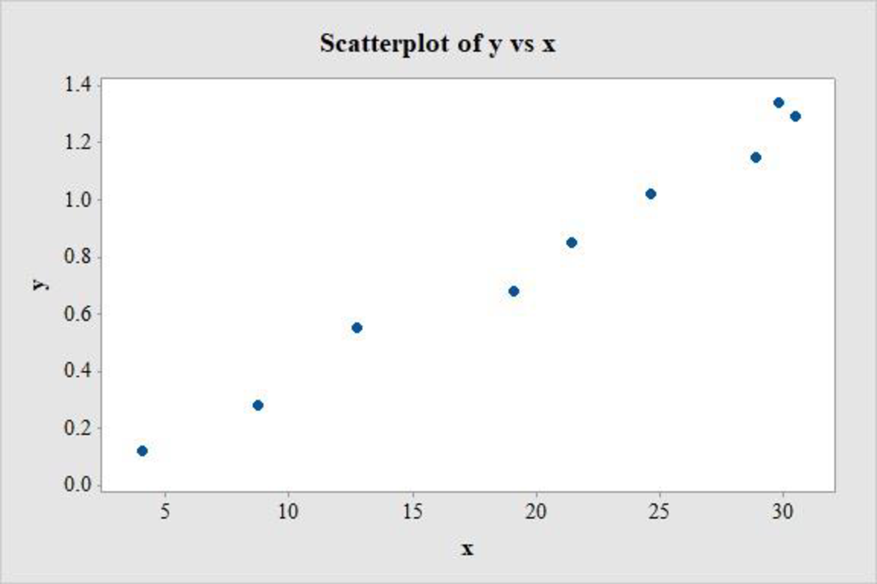
The scatter plot shows no apparent curve and there are no extreme observations. There is no change in the y values as the values of x change and there are no influential points. Therefore, the simple linear regression model seems appropriate for the data set.
b.
Find the equation of the estimated regression line by assuming that the simple linear regression model is appropriate.
Answer to Problem 56CR
The equation of the estimated regression line is,
Explanation of Solution
Calculation:
Regression Analysis:
Software procedure:
Step-by-step procedure to obtain the regression line using MINITAB software:
- Choose Stat > Regression > Regression > Fit Regression Model.
- Under Responses, enter the column of values y.
- Under Continuous predictors, enter the column of values x.
- Click OK.
Output using MINITAB software is given below:
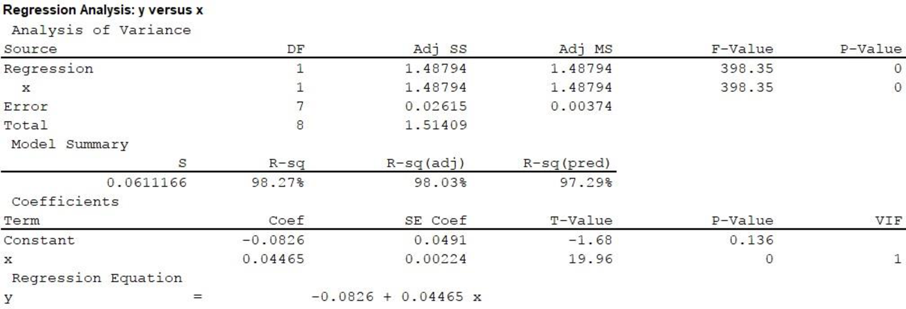
Hence, the equation of the estimated regression line by assuming that the simple linear regression model is appropriate is,
c.
Find how much of the observed variation in peak photo voltage can be explained by the model relationship.
Answer to Problem 56CR
The percentage of observed variation in peak photo voltage that can be explained by the model relationship is 98.3%.
Explanation of Solution
From the Minitab output in Part (b), the value of
This implies that 98.27%, or approximately 98.3% of the observed variation in the dependent variable ‘peak photo voltage’ is being explained by the independent variable ‘percentage of light absorption’ using the simple linear regression model. The change is attributable to the linear relationship between the variables ‘peak photo voltage’ and ‘percentage of light absorption’ and is being explained by the model.
Thus, the percentage of observed variation in peak photo voltage that can be explained by the model relationship is 98.3%.
d.
Predict peak photo voltage when percent absorption is 19.1.
Find the value of the corresponding residual.
Answer to Problem 56CR
The peak voltage when percent absorption is 19.1 is predicted to be 0.770.
The corresponding residual is –0.090.
Explanation of Solution
Calculation:
Predicted value:
The estimated regression equation is,
Hence, the peak voltage when percent absorption is 19.1 is predicted to be 0.770.
Residual:
The formula for residual for response, y and predicted response,
It is given that, when the percentage of light absorption is 19.1, the peak photo voltage is 0.68. Substitute
Hence, the corresponding residual is –0.09.
e.
Explain whether one can agree with the statement that there is a useful linear relationship between the two variables, by carrying out a formal test.
Explanation of Solution
Calculation:
1.
Here,
2.
Null hypothesis:
That is, there is no useful linear relationship between the percentage of light absorption and peak photo voltage.
3.
Alternative hypothesis:
That is, there is a useful linear relationship between the percentage of light absorption and peak photo voltage.
4.
Here, the significance level is assumed to be
5.
Test Statistic:
The formula for test statistic is as follows:
In the formula, b denotes the estimated slope,
6.
Assumption:
The assumption made in Part (b) is that, the simple linear regression model is appropriate.
7.
Calculation:
From the MINITAB output in Part (b), the t-test statistic value for
8.
P-value:
From the MINITAB output in Part (b), the P-value is 0.
9.
Decision rule:
- If P-value is less than or equal to the level of significance, reject the null hypothesis.
- Otherwise, fail to reject the null hypothesis.
10.
Conclusion:
The P-value is 0.
The level of significance is 0.05.
The P-value is less than the level of significance.
That is,
Based on rejection rule, reject the null hypothesis.
Thus, there is convincing evidence of a useful relationship between the percentage of light absorption and peak photo voltage at the 0.05 level of significance.
f.
Obtain an estimate of the average change in peak photo voltage associated with a 1 percentage point increase in light absorption.
Answer to Problem 56CR
The estimate of the average change in peak photo voltage associated with a 1 percentage point increase in light absorption is between 0.039 and 0.050.
Explanation of Solution
Calculation:
From the MINITAB output in Part (b), the value of slope is approximately
Formula for Degrees of freedom:
The formula for degrees of freedom is,
In the formula, n is the total number of observations.
Formula for Confidence interval for
In the formula b denotes the estimated slope and
Degrees of freedom:
The number of data values given are 9, that is
From the Appendix: Table 3 t Critical Values:
- Locate the value 7 in the degrees of freedom (df) column.
- Locate the 0.95 in the row of central area captured.
- The intersecting value that corresponds to the df 7 with confidence level 0.95 is 2.37.
Thus, the critical value for
Confidence interval:
Substitute,
Hence, the 95% confidence interval for estimating the average change in peak photo voltage associated with a 1 percentage point increase in light absorption is
Interpretation:
The 95% confidence interval can be interpreted as: there is 95% confidence that the mean increase in peak photo voltage associated with a 1 percentage point increase in light absorption lies between 0.039 and 0.050.
g.
Obtain an estimate of the average change in peak photo voltage when the percentage of light absorption is 20.
Answer to Problem 56CR
The estimate of the average change in peak photo voltage when the percentage of light absorption is 20 is between 0.762 and 0.859.
Explanation of Solution
Calculation:
The confidence interval for
From the MINITAB output in part (a), the simple linear regression model is
Point estimate:
The point estimate when the percentage of light absorption is 20 is calculated as follows.
Estimated standard deviation:
For the given x values,
Substitute,
Therefore, one can be 95% confident that the mean peak voltage when the percentage of light absorption is 20 is between 0.762 and 0.859.
Want to see more full solutions like this?
Chapter 13 Solutions
Introduction to Statistics and Data Analysis


- Compute the median of the following data. 32, 41, 36, 42, 29, 30, 40, 22, 25, 37arrow_forwardTask Description: Read the following case study and answer the questions that follow. Ella is a 9-year-old third-grade student in an inclusive classroom. She has been diagnosed with Emotional and Behavioural Disorder (EBD). She has been struggling academically and socially due to challenges related to self-regulation, impulsivity, and emotional outbursts. Ella's behaviour includes frequent tantrums, defiance toward authority figures, and difficulty forming positive relationships with peers. Despite her challenges, Ella shows an interest in art and creative activities and demonstrates strong verbal skills when calm. Describe 2 strategies that could be implemented that could help Ella regulate her emotions in class (4 marks) Explain 2 strategies that could improve Ella’s social skills (4 marks) Identify 2 accommodations that could be implemented to support Ella academic progress and provide a rationale for your recommendation.(6 marks) Provide a detailed explanation of 2 ways…arrow_forwardQuestion 2: When John started his first job, his first end-of-year salary was $82,500. In the following years, he received salary raises as shown in the following table. Fill the Table: Fill the following table showing his end-of-year salary for each year. I have already provided the end-of-year salaries for the first three years. Calculate the end-of-year salaries for the remaining years using Excel. (If you Excel answer for the top 3 cells is not the same as the one in the following table, your formula / approach is incorrect) (2 points) Geometric Mean of Salary Raises: Calculate the geometric mean of the salary raises using the percentage figures provided in the second column named “% Raise”. (The geometric mean for this calculation should be nearly identical to the arithmetic mean. If your answer deviates significantly from the mean, it's likely incorrect. 2 points) Starting salary % Raise Raise Salary after raise 75000 10% 7500 82500 82500 4% 3300…arrow_forward
- I need help with this problem and an explanation of the solution for the image described below. (Statistics: Engineering Probabilities)arrow_forwardI need help with this problem and an explanation of the solution for the image described below. (Statistics: Engineering Probabilities)arrow_forward310015 K Question 9, 5.2.28-T Part 1 of 4 HW Score: 85.96%, 49 of 57 points Points: 1 Save of 6 Based on a poll, among adults who regret getting tattoos, 28% say that they were too young when they got their tattoos. Assume that six adults who regret getting tattoos are randomly selected, and find the indicated probability. Complete parts (a) through (d) below. a. Find the probability that none of the selected adults say that they were too young to get tattoos. 0.0520 (Round to four decimal places as needed.) Clear all Final check Feb 7 12:47 US Oarrow_forward
- how could the bar graph have been organized differently to make it easier to compare opinion changes within political partiesarrow_forwardDraw a picture of a normal distribution with mean 70 and standard deviation 5.arrow_forwardWhat do you guess are the standard deviations of the two distributions in the previous example problem?arrow_forward
- Please answer the questionsarrow_forward30. An individual who has automobile insurance from a certain company is randomly selected. Let Y be the num- ber of moving violations for which the individual was cited during the last 3 years. The pmf of Y isy | 1 2 4 8 16p(y) | .05 .10 .35 .40 .10 a.Compute E(Y).b. Suppose an individual with Y violations incurs a surcharge of $100Y^2. Calculate the expected amount of the surcharge.arrow_forward24. An insurance company offers its policyholders a num- ber of different premium payment options. For a ran- domly selected policyholder, let X = the number of months between successive payments. The cdf of X is as follows: F(x)=0.00 : x < 10.30 : 1≤x<30.40 : 3≤ x < 40.45 : 4≤ x <60.60 : 6≤ x < 121.00 : 12≤ x a. What is the pmf of X?b. Using just the cdf, compute P(3≤ X ≤6) and P(4≤ X).arrow_forward
 Functions and Change: A Modeling Approach to Coll...AlgebraISBN:9781337111348Author:Bruce Crauder, Benny Evans, Alan NoellPublisher:Cengage Learning
 College AlgebraAlgebraISBN:9781305115545Author:James Stewart, Lothar Redlin, Saleem WatsonPublisher:Cengage Learning
 Big Ideas Math A Bridge To Success Algebra 1: Stu...AlgebraISBN:9781680331141Author:HOUGHTON MIFFLIN HARCOURTPublisher:Houghton Mifflin Harcourt
 Algebra and Trigonometry (MindTap Course List)AlgebraISBN:9781305071742Author:James Stewart, Lothar Redlin, Saleem WatsonPublisher:Cengage Learning