Chapter 13, Problem 53CR

a.

To determine

Find the expected value of change in biomass concentration associated with a 1-day increase in elapsed time.

Answer to Problem 53CR

A one day increase in elapsed time will decrease the biomass concentration by $\underset{\_}{0.640\text{ g}/{\text{cm}}^{\text{3}}}$.

Explanation of Solution

Calculation:

It is given that y is the green biomass concentration $\left(\text{g}/{\text{cm}}^{\text{3}}\right)$ and x is the elapsed time since snowmelt (days).

The simple linear equation is given as follows:

$\widehat{y}=106.3-0.640x.$

The above regression equation can be interpreted as, 1 unit increase of x will lead to decrease of 0.64 units in y, due to the negative slope of x.

Thus, 1 day increase in elapsed time will decrease the biomass concentration by $\underset{\_}{0.640\text{ g}/{\text{cm}}^{\text{3}}}$.

b.

To determine

Find the predicted value of biomass concentration if elapsed time is 40 days.

Answer to Problem 53CR

The predicted value of biomass concentration for an elapsed time of 40 days is $\underset{\_}{80.7{\text{ g/cm}}^3}.$

Explanation of Solution

Calculation:

From Part (a), the regression equation is given by:

$\widehat{y}=106.3-0.640x.$

Substitute $x=40$ in the above equation. Therefore, the required biomass concentration is obtained as follows:

$\begin{array}{c}\widehat{y}=106.3-0.640x\\ =106.3-0.640\left(40\right)\\ =106.3-25.6\\ =\mathrm{80.7.}\end{array}$

Thus, the predicted value of biomass concentration for elapsed time of 40 days is $\underset{\_}{80.7{\text{ g/cm}}^3}.$

c.

To determine

Check whether there is a linear relationship between the two variables or not.

Answer to Problem 53CR

There is convincing evidence of a useful linear relation between elapsed time and biomass concentration.

Explanation of Solution

Calculation:

It is given that the coefficient of determination $\left(r^2\right)$ is 0.47 and sample size $\left(n\right)$ is 58.

Denote $\beta$ as the regression coefficient.

The null and alternative hypotheses are given by:

$H_0:\beta =0$,

That is, there is no linear relationship between x and y.

$H_{\text{a}}:\beta \ne 0.$

That is, there is a linear relationship between x and y.

Assume that the level of significance for the test is $\alpha =0.05$.

The test statistic for t–test when coefficient of determination is known is given by:

$t=\frac{r}{\sqrt{\frac{1-r^2}{n-2}}}.$

The quantity, $n-2$ is the degrees of freedom.

$\begin{array}{c}r=\sqrt{r^2}\\ =\sqrt{0.47}\\ =\pm \mathrm{0.6856.}\end{array}$

Here, the r value can be considered as negative, because the regression coefficient has negative value. Thus, the acceptable value of r is, $r=0.6856$.

By substituting the values in the test statistic formula, one can get the value of test statistic.

That is,

$\begin{array}{c}t=\frac{r}{\sqrt{\frac{1-r^2}{n-2}}}\\ =\frac{-0.6856}{\sqrt{\frac{1-0.47}{58-2}}}\\ =\frac{-0.6856}{\sqrt{\frac{1-0.47}{56}}}\\ =-\mathrm{7.047.}\end{array}$

Software procedure:

Step-by-step procedure to find the P-value using the MINITAB software:

• Choose Graph > Probability Distribution Plot.
• Choose View Probability > OK.
• From Distribution, choose ‘t’ distribution.
• Enter the Degrees of freedom as 56.
• Click the Shaded Area tab.
• Choose X Value and Both Tails for the region of the curve to shade.
• Enter the X value as –7.047.
• Click OK.

Output obtained using the MINITAB software is represented as follows:

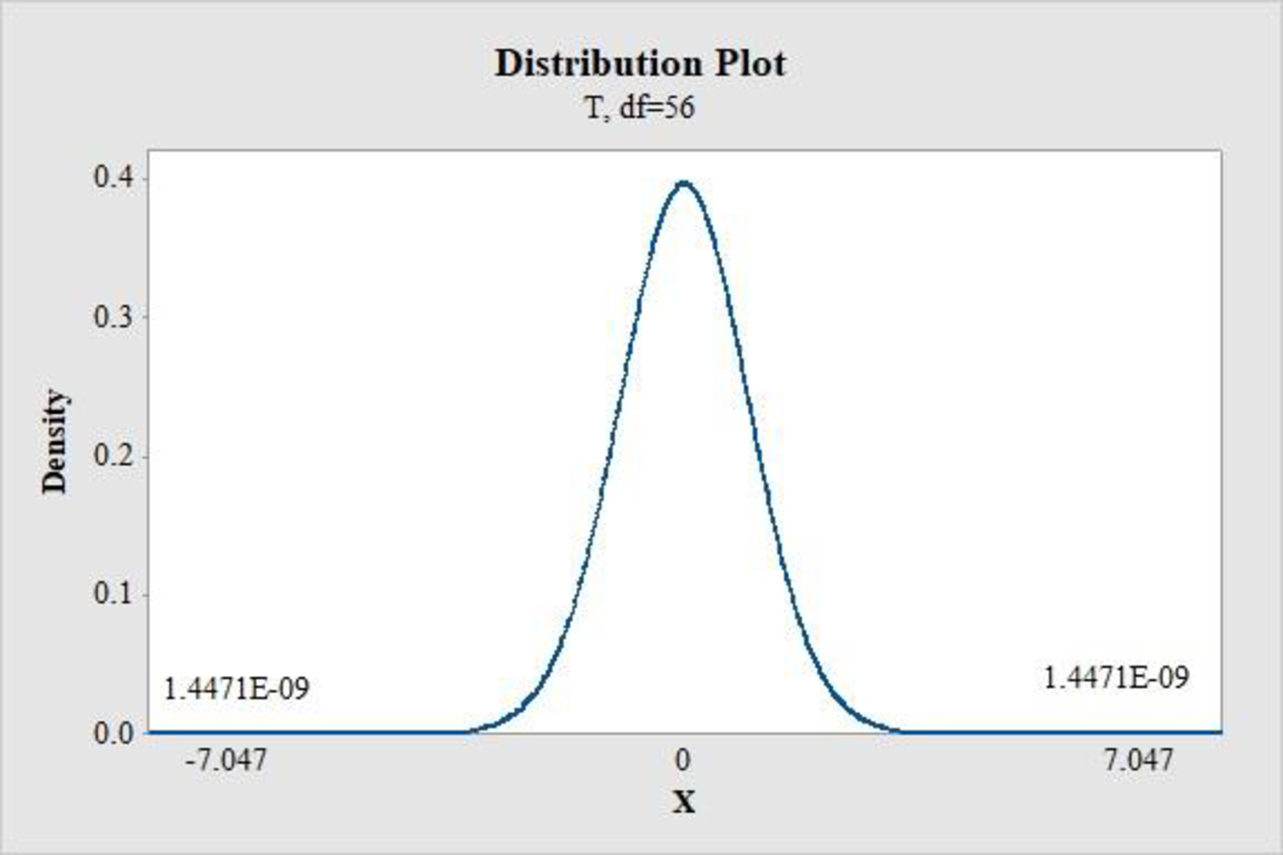
From the above graph, P-value is given by 1.4471E-09, which is approximately 0.

Decision rule:

Reject $H_0$ at level of significance 0.05, if P-value is $\le \mathrm{0.05.}$

Conclusion:

Here, the P-value is 0.

Therefore, the P-value is less than 0.05.

Hence reject $H_0$.

Thus, there is convincing evidence of a useful linear relation between elapsed time and biomass concentration.