Concept explainers
Videos
a.
Construct a
a.
Answer to Problem 48CE
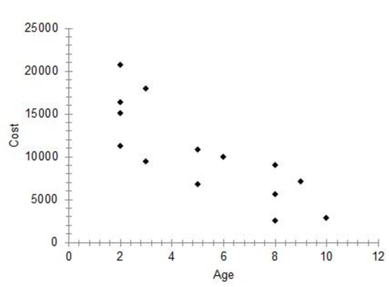
The scatter diagram of the data is as follows:
Explanation of Solution
It is given that ‘Estimated cost’ is the dependent variable.
Step-by-step procedure to obtain the scatterplot using the MegaStat software:
- In an EXCEL sheet enter the data values of x and y.
- Go to Add-Ins > MegaStat >
Correlation/Regression > Scatterplot. - Enter horizontal axis as $B$1:$B$15 and vertical axis as $A$1:$A$15.
- Click on OK.
From the scatterplot of the data, it indicates an inverse relationship.
b.
Find the
b.
Answer to Problem 48CE
The
Explanation of Solution
Step-by-step procedure to obtain the correlation coefficient using the MegaStat software:
- In an EXCEL sheet enter the data values of x and y.
- Go to Add-Ins > MegaStat > Correlation/Regression > Correlation matrix.
- Enter Input
Range as $A$1:$B$15. - Click on OK.
Output obtained using the MegaStat is given as follows:
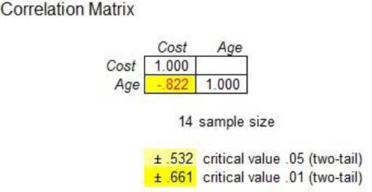
The correlation coefficient is –0.822. Since the correlation coefficient is negative and close to –1, there is a strong
c.
Interpret the slope of the regression equation.
c.
Explanation of Solution
The estimated regression equation is
The interpretation is that for each unit added to age, there is a decrease of $1,534 in cost.
d.
Estimate the cost of a five-year-old car.
d.
Answer to Problem 48CE
The estimated value of cost of a five-year-old car is $10,688.
Explanation of Solution
Substitute x as 5 in the regression equation.
Thus, the estimated value of cost of a five-year-old car is $10,688.
e.
Explain the given portion of the software output.
e.
Explanation of Solution
From the output p-value corresponding to the variable age is 0. That is, the p-value is less than any common level of significance. Thus, the variable age is significant.
f.
Test whether the slope is significant or not.
Interpret the result.
Check whether there is any significant relationship between the two variables.
f.
Answer to Problem 48CE
There is sufficient evidence to conclude that the slope of the regression line is different from zero at the 10% level of significance.
Explanation of Solution
It is given that the regression equation is
From the regression equation, the estimated slope of the regression line is
Let
The given test hypotheses are as follows:
Null hypothesis:
That is, the slope of the regression line is equal to zero.
Alternate hypothesis:
That is, the slope of the regression line is not equal to zero.
It is given that the level of significance is 0.10.
The standard error of
Test statistic:
The t-test statistic is as follows:
Where,
Thus, the following is obtained:
Here, the sample size is
Critical value:
Software procedure:
Step-by-step software procedure to obtain the critical value
- Open an EXCEL file.
- In cell A1, enter the formula “=T.INV(0.05,12)”.
Output obtained using the EXCEL is given as follows:
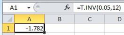
From the EXCEL output, the critical value is –1.782 (
Decision based on critical value:
Reject the null hypothesis, if
Conclusion:
The t-calculated value is 5.01 and the critical value is 1.782.
That is,
Thus, the null hypothesis is rejected.
Hence, there is sufficient evidence to conclude that the slope of the regression line is different from zero at the 10% level of significance.
Since the slope of the regression line is different from zero, there is a relationship between age and cost.
Want to see more full solutions like this?
Chapter 13 Solutions
Loose Leaf for Statistical Techniques in Business and Economics


- Cape Fear Community Colle X ALEKS ALEKS - Dorothy Smith - Sec X www-awu.aleks.com/alekscgi/x/Isl.exe/10_u-IgNslkr7j8P3jH-IQ1w4xc5zw7yX8A9Q43nt5P1XWJWARE... Section 7.1,7.2,7.3 HW 三 Question 21 of 28 (1 point) | Question Attempt: 5 of Unlimited The proportion of phones that have more than 47 apps is 0.8783 Part: 1 / 2 Part 2 of 2 (b) Find the 70th The 70th percentile of the number of apps. Round the answer to two decimal places. percentile of the number of apps is Try again Skip Part Recheck Save 2025 Mcarrow_forwardHi, I need to sort out where I went wrong. So, please us the data attached and run four separate regressions, each using the Recruiters rating as the dependent variable and GMAT, Accept Rate, Salary, and Enrollment, respectively, as a single independent variable. Interpret this equation. Round your answers to four decimal places, if necessary. If your answer is negative number, enter "minus" sign. Equation for GMAT: Ŷ = _______ + _______ GMAT Equation for Accept Rate: Ŷ = _______ + _______ Accept Rate Equation for Salary: Ŷ = _______ + _______ Salary Equation for Enrollment: Ŷ = _______ + _______ Enrollmentarrow_forwardQuestion 21 of 28 (1 point) | Question Attempt: 5 of Unlimited Dorothy ✔ ✓ 12 ✓ 13 ✓ 14 ✓ 15 ✓ 16 ✓ 17 ✓ 18 ✓ 19 ✓ 20 = 21 22 > How many apps? According to a website, the mean number of apps on a smartphone in the United States is 82. Assume the number of apps is normally distributed with mean 82 and standard deviation 30. Part 1 of 2 (a) What proportion of phones have more than 47 apps? Round the answer to four decimal places. The proportion of phones that have more than 47 apps is 0.8783 Part: 1/2 Try again kip Part ی E Recheck == == @ W D 80 F3 151 E R C レ Q FA 975 % T B F5 10 の 000 园 Save For Later Submit Assignment © 2025 McGraw Hill LLC. All Rights Reserved. Terms of Use | Privacy Center | Accessibility Y V& U H J N * 8 M I K O V F10 P = F11 F12 . darrow_forward
- You are provided with data that includes all 50 states of the United States. Your task is to draw a sample of: 20 States using Random Sampling (2 points: 1 for random number generation; 1 for random sample) 10 States using Systematic Sampling (4 points: 1 for random numbers generation; 1 for generating random sample different from the previous answer; 1 for correct K value calculation table; 1 for correct sample drawn by using systematic sampling) (For systematic sampling, do not use the original data directly. Instead, first randomize the data, and then use the randomized dataset to draw your sample. Furthermore, do not use the random list previously generated, instead, generate a new random sample for this part. For more details, please see the snapshot provided at the end.) You are provided with data that includes all 50 states of the United States. Your task is to draw a sample of: o 20 States using Random Sampling (2 points: 1 for random number generation; 1 for random sample) o…arrow_forwardCourse Home ✓ Do Homework - Practice Ques ✓ My Uploads | bartleby + mylab.pearson.com/Student/PlayerHomework.aspx?homeworkId=688589738&questionId=5&flushed=false&cid=8110079¢erwin=yes Online SP 2025 STA 2023-009 Yin = Homework: Practice Questions Exam 3 Question list * Question 3 * Question 4 ○ Question 5 K Concluir atualização: Ava Pearl 04/02/25 9:28 AM HW Score: 71.11%, 12.09 of 17 points ○ Points: 0 of 1 Save Listed in the accompanying table are weights (kg) of randomly selected U.S. Army male personnel measured in 1988 (from "ANSUR I 1988") and different weights (kg) of randomly selected U.S. Army male personnel measured in 2012 (from "ANSUR II 2012"). Assume that the two samples are independent simple random samples selected from normally distributed populations. Do not assume that the population standard deviations are equal. Complete parts (a) and (b). Click the icon to view the ANSUR data. a. Use a 0.05 significance level to test the claim that the mean weight of the 1988…arrow_forwardsolving problem 1arrow_forward
- select bmw stock. you can assume the price of the stockarrow_forwardThis problem is based on the fundamental option pricing formula for the continuous-time model developed in class, namely the value at time 0 of an option with maturity T and payoff F is given by: We consider the two options below: Fo= -rT = e Eq[F]. 1 A. An option with which you must buy a share of stock at expiration T = 1 for strike price K = So. B. An option with which you must buy a share of stock at expiration T = 1 for strike price K given by T K = T St dt. (Note that both options can have negative payoffs.) We use the continuous-time Black- Scholes model to price these options. Assume that the interest rate on the money market is r. (a) Using the fundamental option pricing formula, find the price of option A. (Hint: use the martingale properties developed in the lectures for the stock price process in order to calculate the expectations.) (b) Using the fundamental option pricing formula, find the price of option B. (c) Assuming the interest rate is very small (r ~0), use Taylor…arrow_forwardDiscuss and explain in the picturearrow_forward
- Bob and Teresa each collect their own samples to test the same hypothesis. Bob’s p-value turns out to be 0.05, and Teresa’s turns out to be 0.01. Why don’t Bob and Teresa get the same p-values? Who has stronger evidence against the null hypothesis: Bob or Teresa?arrow_forwardReview a classmate's Main Post. 1. State if you agree or disagree with the choices made for additional analysis that can be done beyond the frequency table. 2. Choose a measure of central tendency (mean, median, mode) that you would like to compute with the data beyond the frequency table. Complete either a or b below. a. Explain how that analysis can help you understand the data better. b. If you are currently unable to do that analysis, what do you think you could do to make it possible? If you do not think you can do anything, explain why it is not possible.arrow_forward0|0|0|0 - Consider the time series X₁ and Y₁ = (I – B)² (I – B³)Xt. What transformations were performed on Xt to obtain Yt? seasonal difference of order 2 simple difference of order 5 seasonal difference of order 1 seasonal difference of order 5 simple difference of order 2arrow_forward
 Glencoe Algebra 1, Student Edition, 9780079039897...AlgebraISBN:9780079039897Author:CarterPublisher:McGraw Hill
 Functions and Change: A Modeling Approach to Coll...AlgebraISBN:9781337111348Author:Bruce Crauder, Benny Evans, Alan NoellPublisher:Cengage Learning
 Algebra and Trigonometry (MindTap Course List)AlgebraISBN:9781305071742Author:James Stewart, Lothar Redlin, Saleem WatsonPublisher:Cengage Learning
 Algebra & Trigonometry with Analytic GeometryAlgebraISBN:9781133382119Author:SwokowskiPublisher:Cengage
 Holt Mcdougal Larson Pre-algebra: Student Edition...AlgebraISBN:9780547587776Author:HOLT MCDOUGALPublisher:HOLT MCDOUGAL