Videos
(a)
To graph: The plot
(a)
Explanation of Solution
Given: The value of
Graph: The plot is drawn by following these steps:
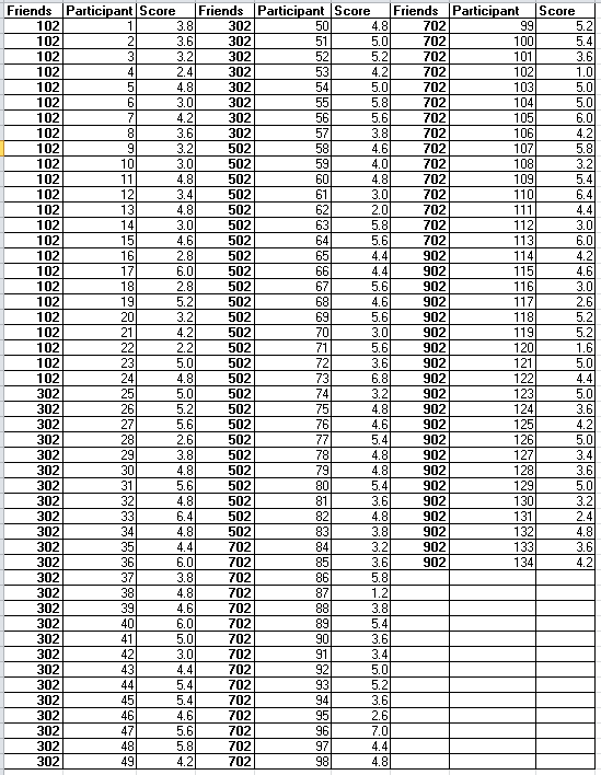
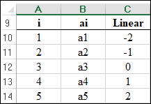
Step 1: Open Excel sheet and write the data value for
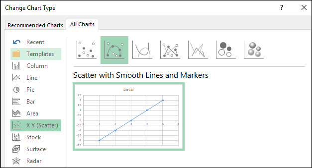
Step 2: INSERT > Recommended Charts > All Charts > Line Chart. The screenshot is shown below:
The plot is obtained as shown below:
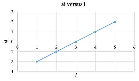
The values chosen for
The contrast can be calculated by the sum of weighted means. If
Interpretation: The value of
(b)
To graph: The plot
(b)
Explanation of Solution
Graph: The plot is drawn by following these steps:
Step 1: Open Excel sheet and write the data value for
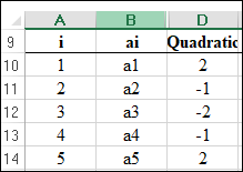
Step 2: INSERT > Recommended Charts > All Charts > Line Chart. The screenshot is shown below:
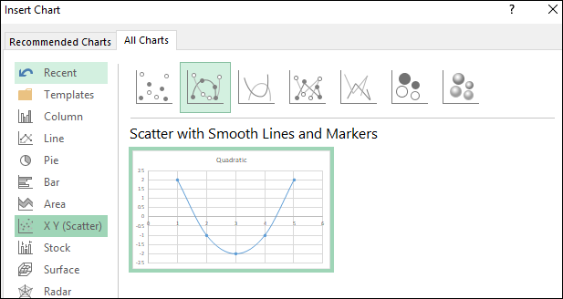
The plot is obtained as shown below:
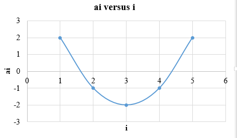
The contrast can be calculated by the sum of weighted means. If
The contrast for means
Interpretation: The value chosen,
(c)
To find: The sample contrast quadratic and cubic trend.
(c)
Answer to Problem 50E
Solution: Contrasts for the quadratic trend can be calculated as:
Contrasts for the cubic trend can be calculated as:
Explanation of Solution
Calculation: To find sample contrasts for quadratic and cubic trend by using the Facebook data as follows:
Contrasts for the quadratic trend can be calculated as:
Contrasts for the cubic trend can be calculated as:
(d)
To test: The hypotheses for the linear, quadratic, and cubic trend.
(d)
Answer to Problem 50E
Solution: The P-values are less than 0
Explanation of Solution
Calculation: To test the null hypothesis, steps are as follows:
Contrasts for the linear trend can be calculated as:
Contrasts for the quadratic trend can be calculated as:
Contrasts for the cubic trend can be calculated as:
The pooled standard deviation is obtained as:
The standard error of linear contrast can be calculated as:
The standard error of quadratic contrast can be calculated as:
The standard error of cubic contrast can be calculated as:
The resultant t statistic values for the linear trend can be calculated as:
The resultant t-statistic values for the quadratic trend can be calculated as:
The resultant t-statistic values for the cubic trend can be calculated as:
The resultant P-values are obtained by using the standard normal distribution table as follows:
Conclusion: The P-values is less than 0
Want to see more full solutions like this?
Chapter 12 Solutions
Introduction to the Practice of Statistics: w/CrunchIt/EESEE Access Card


- K The mean height of women in a country (ages 20-29) is 63.7 inches. A random sample of 65 women in this age group is selected. What is the probability that the mean height for the sample is greater than 64 inches? Assume σ = 2.68. The probability that the mean height for the sample is greater than 64 inches is (Round to four decimal places as needed.)arrow_forwardIn a survey of a group of men, the heights in the 20-29 age group were normally distributed, with a mean of 69.6 inches and a standard deviation of 4.0 inches. A study participant is randomly selected. Complete parts (a) through (d) below. (a) Find the probability that a study participant has a height that is less than 68 inches. The probability that the study participant selected at random is less than 68 inches tall is 0.4. (Round to four decimal places as needed.) 20 2arrow_forwardPEER REPLY 1: Choose a classmate's Main Post and review their decision making process. 1. Choose a risk level for each of the states of nature (assign a probability value to each). 2. Explain why each risk level is chosen. 3. Which alternative do you believe would be the best based on the maximum EMV? 4. Do you feel determining the expected value with perfect information (EVWPI) is worthwhile in this situation? Why or why not?arrow_forward
- Questions An insurance company's cumulative incurred claims for the last 5 accident years are given in the following table: Development Year Accident Year 0 2018 1 2 3 4 245 267 274 289 292 2019 255 276 288 294 2020 265 283 292 2021 263 278 2022 271 It can be assumed that claims are fully run off after 4 years. The premiums received for each year are: Accident Year Premium 2018 306 2019 312 2020 318 2021 326 2022 330 You do not need to make any allowance for inflation. 1. (a) Calculate the reserve at the end of 2022 using the basic chain ladder method. (b) Calculate the reserve at the end of 2022 using the Bornhuetter-Ferguson method. 2. Comment on the differences in the reserves produced by the methods in Part 1.arrow_forwardYou are provided with data that includes all 50 states of the United States. Your task is to draw a sample of: o 20 States using Random Sampling (2 points: 1 for random number generation; 1 for random sample) o 10 States using Systematic Sampling (4 points: 1 for random numbers generation; 1 for random sample different from the previous answer; 1 for correct K value calculation table; 1 for correct sample drawn by using systematic sampling) (For systematic sampling, do not use the original data directly. Instead, first randomize the data, and then use the randomized dataset to draw your sample. Furthermore, do not use the random list previously generated, instead, generate a new random sample for this part. For more details, please see the snapshot provided at the end.) Upload a Microsoft Excel file with two separate sheets. One sheet provides random sampling while the other provides systematic sampling. Excel snapshots that can help you in organizing columns are provided on the next…arrow_forwardThe population mean and standard deviation are given below. Find the required probability and determine whether the given sample mean would be considered unusual. For a sample of n = 65, find the probability of a sample mean being greater than 225 if μ = 224 and σ = 3.5. For a sample of n = 65, the probability of a sample mean being greater than 225 if μ=224 and σ = 3.5 is 0.0102 (Round to four decimal places as needed.)arrow_forward
- ***Please do not just simply copy and paste the other solution for this problem posted on bartleby as that solution does not have all of the parts completed for this problem. Please answer this I will leave a like on the problem. The data needed to answer this question is given in the following link (file is on view only so if you would like to make a copy to make it easier for yourself feel free to do so) https://docs.google.com/spreadsheets/d/1aV5rsxdNjHnkeTkm5VqHzBXZgW-Ptbs3vqwk0SYiQPo/edit?usp=sharingarrow_forwardThe data needed to answer this question is given in the following link (file is on view only so if you would like to make a copy to make it easier for yourself feel free to do so) https://docs.google.com/spreadsheets/d/1aV5rsxdNjHnkeTkm5VqHzBXZgW-Ptbs3vqwk0SYiQPo/edit?usp=sharingarrow_forwardThe following relates to Problems 4 and 5. Christchurch, New Zealand experienced a major earthquake on February 22, 2011. It destroyed 100,000 homes. Data were collected on a sample of 300 damaged homes. These data are saved in the file called CIEG315 Homework 4 data.xlsx, which is available on Canvas under Files. A subset of the data is shown in the accompanying table. Two of the variables are qualitative in nature: Wall construction and roof construction. Two of the variables are quantitative: (1) Peak ground acceleration (PGA), a measure of the intensity of ground shaking that the home experienced in the earthquake (in units of acceleration of gravity, g); (2) Damage, which indicates the amount of damage experienced in the earthquake in New Zealand dollars; and (3) Building value, the pre-earthquake value of the home in New Zealand dollars. PGA (g) Damage (NZ$) Building Value (NZ$) Wall Construction Roof Construction Property ID 1 0.645 2 0.101 141,416 2,826 253,000 B 305,000 B T 3…arrow_forward
- Rose Par posted Apr 5, 2025 9:01 PM Subscribe To: Store Owner From: Rose Par, Manager Subject: Decision About Selling Custom Flower Bouquets Date: April 5, 2025 Our shop, which prides itself on selling handmade gifts and cultural items, has recently received inquiries from customers about the availability of fresh flower bouquets for special occasions. This has prompted me to consider whether we should introduce custom flower bouquets in our shop. We need to decide whether to start offering this new product. There are three options: provide a complete selection of custom bouquets for events like birthdays and anniversaries, start small with just a few ready-made flower arrangements, or do not add flowers. There are also three possible outcomes. First, we might see high demand, and the bouquets could sell quickly. Second, we might have medium demand, with a few sold each week. Third, there might be low demand, and the flowers may not sell well, possibly going to waste. These outcomes…arrow_forwardConsider the state space model X₁ = §Xt−1 + Wt, Yt = AX+Vt, where Xt Є R4 and Y E R². Suppose we know the covariance matrices for Wt and Vt. How many unknown parameters are there in the model?arrow_forwardBusiness Discussarrow_forward
 Big Ideas Math A Bridge To Success Algebra 1: Stu...AlgebraISBN:9781680331141Author:HOUGHTON MIFFLIN HARCOURTPublisher:Houghton Mifflin Harcourt
 Glencoe Algebra 1, Student Edition, 9780079039897...AlgebraISBN:9780079039897Author:CarterPublisher:McGraw Hill
 Algebra & Trigonometry with Analytic GeometryAlgebraISBN:9781133382119Author:SwokowskiPublisher:Cengage
 College Algebra (MindTap Course List)AlgebraISBN:9781305652231Author:R. David Gustafson, Jeff HughesPublisher:Cengage Learning