Chapter 12, Problem 46E

(a)

To determine

To find: The summary from the data.

Answer to Problem 46E

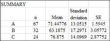
Solution: The summary from the data is as shown below:

Explanation of Solution

Calculation: To draw the inference from the data, use Excel. Steps are provided below:

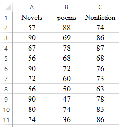
Step 1: Open Excel sheet and write the value for three treatments. The screenshot is shown below:

Step 2: The sample size for “Novels” can be obtained by using the formula $\text{=COUNT(A2:A68)}$. The screenshot is shown below:

The sample size for “Poems” can be obtained by using the formula $\text{=COUNT(B2:B33)}$. The screenshot is shown below:

The sample size for “Nonfiction” can be obtained by using the formula $\text{=COUNT(C2:C25)}$. The screenshot is shown below:

Step 3: The average value for “Novels” can be obtained by using the formula $\text{=AVERAGE(A2:A68)}$. The screenshot is shown below:

The average value for “Poems” can be obtained by using the formula $\text{=AVERAGE(B2:B33)}$. The screenshot is shown below:

The average value for “Nonfiction” can be obtained by using the formula $\text{=AVERAGE(C2:C25)}$. The screenshot is shown below:

Step 4: The standard deviation for “Novels” can be obtained by using the formula $\text{=STDEV(A2:A68)}$. The screenshot is shown below:

The standard deviation for “Poems” can be obtained by using the formula $\text{=STDEV(B2:B33)}$. The screenshot is shown below:

The standard deviation for “Nonfiction” can be obtained by using the formula $\text{=STDEV(C2:C25)}$. The screenshot is shown below:

Step 5: The standard error for “Novels” can be obtained by using the formula $\text{=STDEV(A2:A68)/(SQRT(COUNT(A2:A68)))}$. The screenshot is shown below:

The standard error for “Poems” can be obtained by using the formula $\text{=STDEV(B2:B33)/(SQRT(COUNT(B2:B33)))}$. The screenshot is shown below:

The standard error for “Nonfiction” can be obtained by using the formula $\text{=STDEV(C2:C25)/(SQRT(COUNT(C2:C25)))}$. The screenshot is shown below:

The result is obtained.

The screenshot of the summary of results is shown below:

(b)

To determine

Necessary assumption to carry out ANOVA test.

Answer to Problem 46E

Solution: All the distribution are approximately normal and pooling of standard deviation is applicable.

Explanation of Solution

The necessary assumption is that all the treatment values are approximately normally distributed about their means and the single or pooled standard deviation can be used for all the treatments such that ${\sigma }_{\text{maximum}}<2\times {\sigma }_{\text{minimum}}$.

(c)

To determine

To test: The ANOVA model.

Answer to Problem 46E

Solution: The required ANOVA model is obtained as follows:

$\begin{array}{c}\text{Degree of freedom}=\left(2,117\right)\\ P-\text{value}=0.00088\\ F=7.476\end{array}$

Here, the F value is greater than the F critical value. Hence, the null hypothesis can be rejected significantly.

Explanation of Solution

Calculation: Single factor ANOVA model is performed by following these steps:

Step 1: Open Excel sheet and write the value for three treatments. The screenshot is shown below:

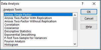
Step 3: Data > Data Analysis > OK. The screenshot is shown below:

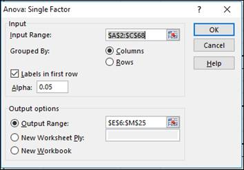
Step 4: Select ANOVA: Single Factor > OK. The screenshot is shown below:

Step 5: Select input range > OK. The screenshot is shown below:

The model is obtained. The screenshot is shown below:

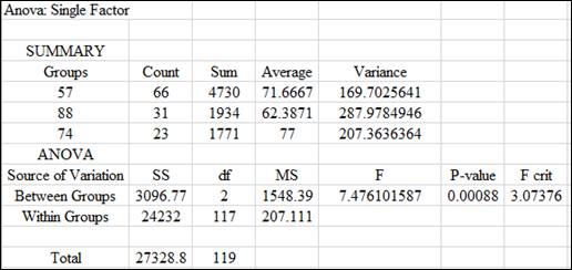
Conclusion: Here, the F value is greater than the F critical. Hence, null hypothesis can be rejected significantly.

(d)

To determine

To test: The contrast to compare the poets with the writers.

Answer to Problem 46E

Solution: The P value is $P\left(t<-3.8\right)<.0001$, which is much less than 0 $.05$ significance level, hence null hypothesis can be rejected at $5\%$ significance level.

Explanation of Solution

A contrast (c) is defined as a combination of population means.

$c={\displaystyle \sum _{i=1}^n{a}_i\times {\mu }_i}$

where ${\displaystyle \sum _{i=1}^n{a}_i}=0$ and ${\mu }_i$ is the sample means.

The null hypothesis, $H_0:c=0$, can be tested by calculating the t statistics as follows:

$t=\frac{c}{S{E}_c}$

where $S{E}_c=s_p\times \sqrt{\frac{{\left(a_1\right)}^2}{n_1}+\frac{{\left(a_2\right)}^2}{n_2}+\frac{{\left(a_3\right)}^2}{n_3}}$ the standard error of contrast and c is the contrast.

The null hypothesis is tested to compare novelists with the nonfiction writers. The following steps are followed with reference to part (c) on excel to test the null hypothesis:

Step 1: Contrast c is calculated as follows:

$\begin{array}{c}c={\displaystyle \sum _{i=1}^n{a}_i\times {\mu }_i}\\ =\left(-0.5\times 71.6667\right)+\left(-0.5\times 77\right)+\left(1\times 62.3871\right)\\ =-11.9462\end{array}$

Step 2: The pooled standard deviation is obtained as follows:

$\begin{array}{c}{s}_p=\sqrt{\frac{\left(n_1-1\right)s_1^2+\left(n_2-1\right)s_2^2+\left(n_3-1\right)s_3^2}{n_1+n_2+n_3-3}}\\ =\sqrt{\frac{\left(66-1\right)169.703+\left(23-1\right)207.364+\left(31-1\right)287.978}{66+23+31-3}}\\ =14.4766\end{array}$

Step 3: Standard error of contrast is obtained as follows:

$\begin{array}{c}S{E}_c=s_p\times \sqrt{\frac{{\left(-0.5\right)}^2}{n_1}+\frac{{\left(-0.5\right)}^2}{n_2}+\frac{{\left(1\right)}^2}{n_3}}\\ =13.3875\times \sqrt{\frac{{\left(-0.5\right)}^2}{66}+\frac{{\left(-0.5\right)}^2}{23}+\frac{{\left(1\right)}^2}{31}}\\ =3.13564\end{array}$

Step 4: The resultant t statistic can be calculated as follows:

$\begin{array}{c}t=\frac{c}{S{E}_c}\\ =\frac{-11.9462}{3.13564}\\ =-3.80983\end{array}$

(e)

To determine

To test: A contrast to compare the novelists with the nonfiction writers.

Answer to Problem 46E

Solution: The p- value is $P\left(t<-1.65\right)=.0505$ that is approximately equal to 0.05 significance level, hence null hypothesis can be rejected at 5% significance level.

Explanation of Solution

The null hypothesis is tested to compare novelists with the nonfiction writers. The following steps are followed with reference to part (c) on excel to test the null hypothesis:

Step 1: Contrast c is calculated as follows:

$\begin{array}{c}c={\displaystyle \sum _{i=1}^n{a}_i\times {\mu }_i}\\ =\left(-0.5\times 71.6667\right)+\left(0.5\times 77\right)\\ =2.66667\end{array}$

Step 2: The pooled standard deviation is obtained as follows:

$\begin{array}{c}{s}_p=\sqrt{\frac{\left(n_1-1\right)s_1^2+\left(n_2-1\right)s_2^2}{n_1+n_2-2}}\\ =\sqrt{\frac{\left(66-1\right)169.703+\left(23-1\right)14.4001}{66+23-2}}\\ =13.3875\end{array}$

Step 3: Standard error of contrast can be calculated as follows:

$\begin{array}{c}S{E}_c=s_p\times \sqrt{\frac{{\left(-0.5\right)}^2}{n_1}+\frac{{\left(-0.5\right)}^2}{n_2}}\\ =13.3875\times \sqrt{\frac{{\left(-0.5\right)}^2}{66}+\frac{{\left(-0.5\right)}^2}{23}}\\ =1.6208\end{array}$

Step 4: The resultant t statistic can be calculated as follows:

$\begin{array}{c}t=\frac{c}{S{E}_c}\\ =\frac{2.66667}{1.6208}\\ =1.64528\end{array}$

Conclusion: The p- value is $P\left(t<-1.65\right)=.0505$ that is approximately equal to 0.05 significance level, hence null hypothesis can be rejected at 5% significance level.

(f)

To determine

To test: The multiple comparison t test.

Answer to Problem 46E

Solution: The poem’s mean is significantly different from other means.

Explanation of Solution

To perform the multiple comparison t-test, there are three possible combinations that are novels versus poems, poems versus nonfiction, and novels versus nonfiction. The steps to be followed on excel to obtain the multiple comparison t test are mentioned below.

Calculation:

Multiple comparison t-test is performed by following these steps:

Step 1: Open Excel sheet and write the value for three treatments. The screenshot is shown below:

Step 2: Data > Data Analysis > OK. The screenshot is shown below:

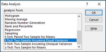
Step 3: Select t-test: Two-Sample Assuming Equal Variances > OK. The screenshot is shown below:

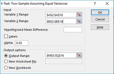
Step 4: Select input range > OK. The screenshot is shown below:

Step 5: Repeat step 5 to compare low dose versus high dose and control versus high dose.

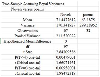
The result for comparison of novels versus poems is obtained as follows:

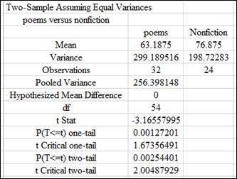
The result for comparison of poems versus nonfiction is obtained as follows:

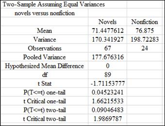
The result for comparison of novels versus nonfiction is obtained as follows:

Conclusion: From the above comparison, the P value for two-tail for poems versus novels and poems versus nonfiction is less than 0.05 at 5% significance level. Hence, poem’s mean is significantly different from other means.