Concept explainers
Videos
(a)
To find: The fitted data and the residuals. Also, generate the
(a)
Answer to Problem 22E
Solution: The residuals of the provided data is scattered symmetrically above and below the zero and there is no extreme outlier.
Explanation of Solution
Given: The data provided in the Facebook friends study as,
| Friends | Participant | Score |
| 102 | 1 | 3.8 |
| 102 | 2 | 3.6 |
| 102 | 3 | 3.2 |
| 102 | 4 | 2.4 |
| 102 | 5 | 4.8 |
| 102 | 6 | 3.0 |
| 102 | 7 | 4.2 |
| 102 | 8 | 3.6 |
| 102 | 9 | 3.2 |
| 102 | 10 | 3.0 |
| 102 | 11 | 4.8 |
| 102 | 12 | 3.4 |
| 102 | 13 | 4.8 |
| 102 | 14 | 3.0 |
| 102 | 15 | 4.6 |
| 102 | 16 | 2.8 |
| 102 | 17 | 6.0 |
| 102 | 18 | 2.8 |
| 102 | 19 | 5.2 |
| 102 | 20 | 3.2 |
| 102 | 21 | 4.2 |
| 102 | 22 | 2.2 |
| 102 | 23 | 5.0 |
| 102 | 24 | 4.8 |
| 302 | 25 | 5.0 |
| 302 | 26 | 5.2 |
| 302 | 27 | 5.6 |
| 302 | 28 | 2.6 |
| 302 | 29 | 3.8 |
| 302 | 30 | 4.8 |
| 302 | 31 | 5.6 |
| 302 | 32 | 4.8 |
| 302 | 33 | 6.4 |
| 302 | 34 | 4.8 |
| 302 | 35 | 4.4 |
| 302 | 36 | 6.0 |
| 302 | 37 | 3.8 |
| 302 | 38 | 4.8 |
| 302 | 39 | 4.6 |
| 302 | 40 | 6.0 |
| 302 | 41 | 5.0 |
| 302 | 42 | 3.0 |
| 302 | 43 | 4.4 |
| 302 | 44 | 5.4 |
| 302 | 45 | 5.4 |
| 302 | 46 | 4.6 |
| 302 | 47 | 5.6 |
| 302 | 48 | 5.8 |
| 302 | 49 | 4.2 |
| 302 | 50 | 4.8 |
| 302 | 51 | 5.0 |
| 302 | 52 | 5.2 |
| 302 | 53 | 4.2 |
| 302 | 54 | 5.0 |
| 302 | 55 | 5.8 |
| 302 | 56 | 5.6 |
| 302 | 57 | 3.8 |
| 502 | 58 | 4.6 |
| 502 | 59 | 4.0 |
| 502 | 60 | 4.8 |
| 502 | 61 | 3.0 |
| 502 | 62 | 2.0 |
| 502 | 63 | 5.8 |
| 502 | 64 | 5.6 |
| 502 | 65 | 4.4 |
| 502 | 66 | 4.4 |
| 502 | 67 | 5.6 |
| 502 | 68 | 4.6 |
| 502 | 69 | 5.6 |
| 502 | 70 | 3.0 |
| 502 | 71 | 5.6 |
| 502 | 72 | 3.6 |
| 502 | 73 | 6.8 |
| 502 | 74 | 3.2 |
| 502 | 75 | 4.8 |
| 502 | 76 | 4.6 |
| 502 | 77 | 5.4 |
| 502 | 78 | 4.8 |
| 502 | 79 | 4.8 |
| 502 | 80 | 5.4 |
| 502 | 81 | 3.6 |
| 502 | 82 | 4.8 |
| 502 | 83 | 3.8 |
| 702 | 84 | 3.2 |
| 702 | 85 | 3.6 |
| 702 | 86 | 5.8 |
| 702 | 87 | 1.2 |
| 702 | 88 | 3.8 |
| 702 | 89 | 5.4 |
| 702 | 90 | 3.6 |
| 702 | 91 | 3.4 |
| 702 | 92 | 5.0 |
| 702 | 93 | 5.2 |
| 702 | 94 | 3.6 |
| 702 | 95 | 2.6 |
| 702 | 96 | 7.0 |
| 702 | 97 | 4.4 |
| 702 | 98 | 4.8 |
| 702 | 99 | 5.2 |
| 702 | 100 | 5.4 |
| 702 | 101 | 3.6 |
| 702 | 102 | 1.0 |
| 702 | 103 | 5.0 |
| 702 | 104 | 5.0 |
| 702 | 105 | 6.0 |
| 702 | 106 | 4.2 |
| 702 | 107 | 5.8 |
| 702 | 108 | 3.2 |
| 702 | 109 | 5.4 |
| 702 | 110 | 6.4 |
| 702 | 111 | 4.4 |
| 702 | 112 | 3.0 |
| 702 | 113 | 6.0 |
| 902 | 114 | 4.2 |
| 902 | 115 | 4.6 |
| 902 | 116 | 3.0 |
| 902 | 117 | 2.6 |
| 902 | 118 | 5.2 |
| 902 | 119 | 5.2 |
| 902 | 120 | 1.6 |
| 902 | 121 | 5.0 |
| 902 | 122 | 4.4 |
| 902 | 123 | 5.0 |
| 902 | 124 | 3.6 |
| 902 | 125 | 4.2 |
| 902 | 126 | 5.0 |
| 902 | 127 | 3.4 |
| 902 | 128 | 3.6 |
| 902 | 129 | 5.0 |
| 902 | 130 | 3.2 |
| 902 | 131 | 2.4 |
| 902 | 132 | 4.8 |
| 902 | 133 | 3.6 |
| 902 | 134 | 4.2 |
Calculation:
Use Minitab to find the residuals, of the provided data as below:
Step1: Enter the provided data in the worksheet.
Step2: Select stat >ANOVA>one-way analysis of variance.
Step3: Select Score in the Response and Friends in the Factor.
Step4: Click on Graphs and select the Residual verses fitand then press OK.
Step5: Select Store residual and Store fit.
Step6: Press OK.
Theobtained output of fitted data and the residual stored in the data file as below:
| Friends | Participant | Score | RESI1 | FITS1 |
| 102 | 1 | 3.8 | -0.01667 | 3.816667 |
| 102 | 2 | 3.6 | -0.21667 | 3.816667 |
| 102 | 3 | 3.2 | -0.61667 | 3.816667 |
| 102 | 4 | 2.4 | -1.41667 | 3.816667 |
| 102 | 5 | 4.8 | 0.983333 | 3.816667 |
| 102 | 6 | 3.0 | -0.81667 | 3.816667 |
| 102 | 7 | 4.2 | 0.383333 | 3.816667 |
| 102 | 8 | 3.6 | -0.21667 | 3.816667 |
| 102 | 9 | 3.2 | -0.61667 | 3.816667 |
| 102 | 10 | 3.0 | -0.81667 | 3.816667 |
| 102 | 11 | 4.8 | 0.983333 | 3.816667 |
| 102 | 12 | 3.4 | -0.41667 | 3.816667 |
| 102 | 13 | 4.8 | 0.983333 | 3.816667 |
| 102 | 14 | 3.0 | -0.81667 | 3.816667 |
| 102 | 15 | 4.6 | 0.783333 | 3.816667 |
| 102 | 16 | 2.8 | -1.01667 | 3.816667 |
| 102 | 17 | 6.0 | 2.183333 | 3.816667 |
| 102 | 18 | 2.8 | -1.01667 | 3.816667 |
| 102 | 19 | 5.2 | 1.383333 | 3.816667 |
| 102 | 20 | 3.2 | -0.61667 | 3.816667 |
| 102 | 21 | 4.2 | 0.383333 | 3.816667 |
| 102 | 22 | 2.2 | -1.61667 | 3.816667 |
| 102 | 23 | 5.0 | 1.183333 | 3.816667 |
| 102 | 24 | 4.8 | 0.983333 | 3.816667 |
| 302 | 25 | 5.0 | 0.121212 | 4.878788 |
| 302 | 26 | 5.2 | 0.321212 | 4.878788 |
| 302 | 27 | 5.6 | 0.721212 | 4.878788 |
| 302 | 28 | 2.6 | -2.27879 | 4.878788 |
| 302 | 29 | 3.8 | -1.07879 | 4.878788 |
| 302 | 30 | 4.8 | -0.07879 | 4.878788 |
| 302 | 31 | 5.6 | 0.721212 | 4.878788 |
| 302 | 32 | 4.8 | -0.07879 | 4.878788 |
| 302 | 33 | 6.4 | 1.521212 | 4.878788 |
| 302 | 34 | 4.8 | -0.07879 | 4.878788 |
| 302 | 35 | 4.4 | -0.47879 | 4.878788 |
| 302 | 36 | 6.0 | 1.121212 | 4.878788 |
| 302 | 37 | 3.8 | -1.07879 | 4.878788 |
| 302 | 38 | 4.8 | -0.07879 | 4.878788 |
| 302 | 39 | 4.6 | -0.27879 | 4.878788 |
| 302 | 40 | 6.0 | 1.121212 | 4.878788 |
| 302 | 41 | 5.0 | 0.121212 | 4.878788 |
| 302 | 42 | 3.0 | -1.87879 | 4.878788 |
| 302 | 43 | 4.4 | -0.47879 | 4.878788 |
| 302 | 44 | 5.4 | 0.521212 | 4.878788 |
| 302 | 45 | 5.4 | 0.521212 | 4.878788 |
| 302 | 46 | 4.6 | -0.27879 | 4.878788 |
| 302 | 47 | 5.6 | 0.721212 | 4.878788 |
| 302 | 48 | 5.8 | 0.921212 | 4.878788 |
| 302 | 49 | 4.2 | -0.67879 | 4.878788 |
| 302 | 50 | 4.8 | -0.07879 | 4.878788 |
| 302 | 51 | 5.0 | 0.121212 | 4.878788 |
| 302 | 52 | 5.2 | 0.321212 | 4.878788 |
| 302 | 53 | 4.2 | -0.67879 | 4.878788 |
| 302 | 54 | 5.0 | 0.121212 | 4.878788 |
| 302 | 55 | 5.8 | 0.921212 | 4.878788 |
| 302 | 56 | 5.6 | 0.721212 | 4.878788 |
| 302 | 57 | 3.8 | -1.07879 | 4.878788 |
| 502 | 58 | 4.6 | 0.038462 | 4.561538 |
| 502 | 59 | 4.0 | -0.56154 | 4.561538 |
| 502 | 60 | 4.8 | 0.238462 | 4.561538 |
| 502 | 61 | 3.0 | -1.56154 | 4.561538 |
| 502 | 62 | 2.0 | -2.56154 | 4.561538 |
| 502 | 63 | 5.8 | 1.238462 | 4.561538 |
| 502 | 64 | 5.6 | 1.038462 | 4.561538 |
| 502 | 65 | 4.4 | -0.16154 | 4.561538 |
| 502 | 66 | 4.4 | -0.16154 | 4.561538 |
| 502 | 67 | 5.6 | 1.038462 | 4.561538 |
| 502 | 68 | 4.6 | 0.038462 | 4.561538 |
| 502 | 69 | 5.6 | 1.038462 | 4.561538 |
| 502 | 70 | 3.0 | -1.56154 | 4.561538 |
| 502 | 71 | 5.6 | 1.038462 | 4.561538 |
| 502 | 72 | 3.6 | -0.96154 | 4.561538 |
| 502 | 73 | 6.8 | 2.238462 | 4.561538 |
| 502 | 74 | 3.2 | -1.36154 | 4.561538 |
| 502 | 75 | 4.8 | 0.238462 | 4.561538 |
| 502 | 76 | 4.6 | 0.038462 | 4.561538 |
| 502 | 77 | 5.4 | 0.838462 | 4.561538 |
| 502 | 78 | 4.8 | 0.238462 | 4.561538 |
| 502 | 79 | 4.8 | 0.238462 | 4.561538 |
| 502 | 80 | 5.4 | 0.838462 | 4.561538 |
| 502 | 81 | 3.6 | -0.96154 | 4.561538 |
| 502 | 82 | 4.8 | 0.238462 | 4.561538 |
| 502 | 83 | 3.8 | -0.76154 | 4.561538 |
| 702 | 84 | 3.2 | -1.20667 | 4.406667 |
| 702 | 85 | 3.6 | -0.80667 | 4.406667 |
| 702 | 86 | 5.8 | 1.393333 | 4.406667 |
| 702 | 87 | 1.2 | -3.20667 | 4.406667 |
| 702 | 88 | 3.8 | -0.60667 | 4.406667 |
| 702 | 89 | 5.4 | 0.993333 | 4.406667 |
| 702 | 90 | 3.6 | -0.80667 | 4.406667 |
| 702 | 91 | 3.4 | -1.00667 | 4.406667 |
| 702 | 92 | 5.0 | 0.593333 | 4.406667 |
| 702 | 93 | 5.2 | 0.793333 | 4.406667 |
| 702 | 94 | 3.6 | -0.80667 | 4.406667 |
| 702 | 95 | 2.6 | -1.80667 | 4.406667 |
| 702 | 96 | 7.0 | 2.593333 | 4.406667 |
| 702 | 97 | 4.4 | -0.00667 | 4.406667 |
| 702 | 98 | 4.8 | 0.393333 | 4.406667 |
| 702 | 99 | 5.2 | 0.793333 | 4.406667 |
| 702 | 100 | 5.4 | 0.993333 | 4.406667 |
| 702 | 101 | 3.6 | -0.80667 | 4.406667 |
| 702 | 102 | 1.0 | -3.40667 | 4.406667 |
| 702 | 103 | 5.0 | 0.593333 | 4.406667 |
| 702 | 104 | 5.0 | 0.593333 | 4.406667 |
| 702 | 105 | 6.0 | 1.593333 | 4.406667 |
| 702 | 106 | 4.2 | -0.20667 | 4.406667 |
| 702 | 107 | 5.8 | 1.393333 | 4.406667 |
| 702 | 108 | 3.2 | -1.20667 | 4.406667 |
| 702 | 109 | 5.4 | 0.993333 | 4.406667 |
| 702 | 110 | 6.4 | 1.993333 | 4.406667 |
| 702 | 111 | 4.4 | -0.00667 | 4.406667 |
| 702 | 112 | 3.0 | -1.40667 | 4.406667 |
| 702 | 113 | 6.0 | 1.593333 | 4.406667 |
| 902 | 114 | 4.2 | 0.209524 | 3.990476 |
| 902 | 115 | 4.6 | 0.609524 | 3.990476 |
| 902 | 116 | 3.0 | -0.99048 | 3.990476 |
| 902 | 117 | 2.6 | -1.39048 | 3.990476 |
| 902 | 118 | 5.2 | 1.209524 | 3.990476 |
| 902 | 119 | 5.2 | 1.209524 | 3.990476 |
| 902 | 120 | 1.6 | -2.39048 | 3.990476 |
| 902 | 121 | 5.0 | 1.009524 | 3.990476 |
| 902 | 122 | 4.4 | 0.409524 | 3.990476 |
| 902 | 123 | 5.0 | 1.009524 | 3.990476 |
| 902 | 124 | 3.6 | -0.39048 | 3.990476 |
| 902 | 125 | 4.2 | 0.209524 | 3.990476 |
| 902 | 126 | 5.0 | 1.009524 | 3.990476 |
| 902 | 127 | 3.4 | -0.59048 | 3.990476 |
| 902 | 128 | 3.6 | -0.39048 | 3.990476 |
| 902 | 129 | 5.0 | 1.009524 | 3.990476 |
| 902 | 130 | 3.2 | -0.79048 | 3.990476 |
| 902 | 131 | 2.4 | -1.59048 | 3.990476 |
| 902 | 132 | 4.8 | 0.809524 | 3.990476 |
| 902 | 133 | 3.6 | -0.39048 | 3.990476 |
| 902 | 134 | 4.2 | 0.209524 | 3.990476 |
The scatterplot of the residuals versus the group variable is,
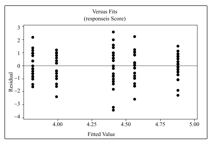
Interpretation: From the above graph, it is observed that the scatter plot of the residuals is symmetrically scattered below and above the zero and there are two outliers below the zero but these are not the extreme outliers.
(b)
Whether the spread of the residual of each group is relatively equal or not.
(b)
Answer to Problem 22E
Solution: Yes, the spread of the residual of each group is relatively equal.
Explanation of Solution
From the scatterplot of the residuals versus the group variables in part (a), it is observed that the residuals are symmetrically scattered below and above the zero. It implies that the spread of the residual of each group is relatively equal.
(c)
To graph: The Normal quantile plot of the residuals obtained in part (a) and identify whether it is normal or not.
(c)
Explanation of Solution
Graph:
Use Minitab to graph the Normal quantile plot as below:
Step1: Enter the provided data in the worksheet.
Step2: Select stat> ANOVA>one-way analysis of variance.
Step3: Select Score in the Response and Friends in the Factor.
Step4: Click on Graphs and select the Normal plot of residuals and then press OK.
Step5: Press OK.
The obtained graph is,
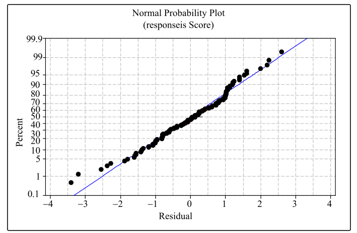
Interpretation: From the obtained graph, it is observed that the normal quantile plot is nearly fitted to the line. Hence, the residual is approximately normal.
Want to see more full solutions like this?
Chapter 12 Solutions
Introduction to the Practice of Statistics: w/CrunchIt/EESEE Access Card


- The population mean and standard deviation are given below. Find the required probability and determine whether the given sample mean would be considered unusual. For a sample of n = 65, find the probability of a sample mean being greater than 225 if μ = 224 and σ = 3.5. For a sample of n = 65, the probability of a sample mean being greater than 225 if μ=224 and σ = 3.5 is 0.0102 (Round to four decimal places as needed.)arrow_forward***Please do not just simply copy and paste the other solution for this problem posted on bartleby as that solution does not have all of the parts completed for this problem. Please answer this I will leave a like on the problem. The data needed to answer this question is given in the following link (file is on view only so if you would like to make a copy to make it easier for yourself feel free to do so) https://docs.google.com/spreadsheets/d/1aV5rsxdNjHnkeTkm5VqHzBXZgW-Ptbs3vqwk0SYiQPo/edit?usp=sharingarrow_forwardThe data needed to answer this question is given in the following link (file is on view only so if you would like to make a copy to make it easier for yourself feel free to do so) https://docs.google.com/spreadsheets/d/1aV5rsxdNjHnkeTkm5VqHzBXZgW-Ptbs3vqwk0SYiQPo/edit?usp=sharingarrow_forward
- The following relates to Problems 4 and 5. Christchurch, New Zealand experienced a major earthquake on February 22, 2011. It destroyed 100,000 homes. Data were collected on a sample of 300 damaged homes. These data are saved in the file called CIEG315 Homework 4 data.xlsx, which is available on Canvas under Files. A subset of the data is shown in the accompanying table. Two of the variables are qualitative in nature: Wall construction and roof construction. Two of the variables are quantitative: (1) Peak ground acceleration (PGA), a measure of the intensity of ground shaking that the home experienced in the earthquake (in units of acceleration of gravity, g); (2) Damage, which indicates the amount of damage experienced in the earthquake in New Zealand dollars; and (3) Building value, the pre-earthquake value of the home in New Zealand dollars. PGA (g) Damage (NZ$) Building Value (NZ$) Wall Construction Roof Construction Property ID 1 0.645 2 0.101 141,416 2,826 253,000 B 305,000 B T 3…arrow_forwardRose Par posted Apr 5, 2025 9:01 PM Subscribe To: Store Owner From: Rose Par, Manager Subject: Decision About Selling Custom Flower Bouquets Date: April 5, 2025 Our shop, which prides itself on selling handmade gifts and cultural items, has recently received inquiries from customers about the availability of fresh flower bouquets for special occasions. This has prompted me to consider whether we should introduce custom flower bouquets in our shop. We need to decide whether to start offering this new product. There are three options: provide a complete selection of custom bouquets for events like birthdays and anniversaries, start small with just a few ready-made flower arrangements, or do not add flowers. There are also three possible outcomes. First, we might see high demand, and the bouquets could sell quickly. Second, we might have medium demand, with a few sold each week. Third, there might be low demand, and the flowers may not sell well, possibly going to waste. These outcomes…arrow_forwardConsider the state space model X₁ = §Xt−1 + Wt, Yt = AX+Vt, where Xt Є R4 and Y E R². Suppose we know the covariance matrices for Wt and Vt. How many unknown parameters are there in the model?arrow_forward
- Business Discussarrow_forwardYou want to obtain a sample to estimate the proportion of a population that possess a particular genetic marker. Based on previous evidence, you believe approximately p∗=11% of the population have the genetic marker. You would like to be 90% confident that your estimate is within 0.5% of the true population proportion. How large of a sample size is required?n = (Wrong: 10,603) Do not round mid-calculation. However, you may use a critical value accurate to three decimal places.arrow_forward2. [20] Let {X1,..., Xn} be a random sample from Ber(p), where p = (0, 1). Consider two estimators of the parameter p: 1 p=X_and_p= n+2 (x+1). For each of p and p, find the bias and MSE.arrow_forward
- 1. [20] The joint PDF of RVs X and Y is given by xe-(z+y), r>0, y > 0, fx,y(x, y) = 0, otherwise. (a) Find P(0X≤1, 1arrow_forward4. [20] Let {X1,..., X} be a random sample from a continuous distribution with PDF f(x; 0) = { Axe 5 0, x > 0, otherwise. where > 0 is an unknown parameter. Let {x1,...,xn} be an observed sample. (a) Find the value of c in the PDF. (b) Find the likelihood function of 0. (c) Find the MLE, Ô, of 0. (d) Find the bias and MSE of 0.arrow_forward3. [20] Let {X1,..., Xn} be a random sample from a binomial distribution Bin(30, p), where p (0, 1) is unknown. Let {x1,...,xn} be an observed sample. (a) Find the likelihood function of p. (b) Find the MLE, p, of p. (c) Find the bias and MSE of p.arrow_forwardarrow_back_iosSEE MORE QUESTIONSarrow_forward_ios
 Big Ideas Math A Bridge To Success Algebra 1: Stu...AlgebraISBN:9781680331141Author:HOUGHTON MIFFLIN HARCOURTPublisher:Houghton Mifflin Harcourt
 Glencoe Algebra 1, Student Edition, 9780079039897...AlgebraISBN:9780079039897Author:CarterPublisher:McGraw Hill
 Functions and Change: A Modeling Approach to Coll...AlgebraISBN:9781337111348Author:Bruce Crauder, Benny Evans, Alan NoellPublisher:Cengage Learning
 Holt Mcdougal Larson Pre-algebra: Student Edition...AlgebraISBN:9780547587776Author:HOLT MCDOUGALPublisher:HOLT MCDOUGAL
 College AlgebraAlgebraISBN:9781305115545Author:James Stewart, Lothar Redlin, Saleem WatsonPublisher:Cengage Learning