Videos
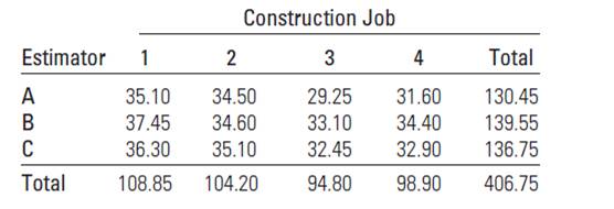
Bidding on Construction Jobs A building contractor employs three construction engineers. A, B, and C, to estimate and bid on jobs. To determine whether one tends to be a more conservative (or liberal) estimator than the others, the contractor selects four projected construction jobs and has each estimator independently estimate the cost (in dollars per square foot) of each job. The data are shown in the table: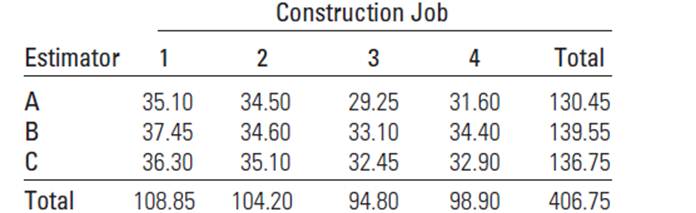
Analyze the experiment using the appropriate methods. Identity the blocks and treatments, and investigate any possible differences in treatment means. If any differences exist, use an appropriate method to specifically identity where the differences lie. Has blocking been effective in this experiment? What are the practical implications of the experiment’? Present your results in the form of a report.
To find: the blocks and treatments, whether the blocking iseffective, the practical implications.
Answer to Problem 11.41E
There is not sufficient evidence to support the claim that there are differences in the mean cost for the different construction jobs and there is not sufficient evidence to support the claim that there are differences in the mean cost for the different estimators.
Blocking was not effective.
The practical implications are that it does not matter which estimator is used, as we will always obtain the same mean cost.
Explanation of Solution
Given:
Calculation:
The necessary sum is,
The treatments are the estimators, while the blocks are the construction jobs, because we suspect that there could be a difference in the cost for each job.
The value of
The value of
The value of
The value of
Total
The value of the test statistic is calculated as
| Source | SS | MS | F | |
| Construction job | 2 | 65.86 | 32.93 | 0.9027 |
| Estimator | 3 | 174.77 | 58.26 | 1.5970 |
| Error | 6 | 218.87 | 36.48 | |
| total | 11 | 459.57 |
Construction job:
The P-value is the number in the row title of the F-distribution table in the appendix containing the F-value
If the P-value is less than the significance level, then reject the null hypothesis.
There is not sufficient evidence to support the claim that there are differences in the mean cost for the different construction jobs.
Blocking was not effective, because there was no significant difference in the mean cost for the different construction jobs.
Estimator:
The P-value is the number in the row title of the F-distribution table in the appendix containing the F-value
If the P-value is less than the significance level, then reject the null hypothesis.
There is not sufficient evidence to support the claim that there are differences in the mean cost for the different estimators.
The practical implications are that it does not matter which estimator is used, as we will always obtain the same mean cost.
Conclusions:
Therefore,treatments: estimator A, B, C
Block: Construction job 1, 2, 3, 4
There is not sufficient evidence to support the claim that there are differences in the mean cost for the different construction jobs and there is not sufficient evidence to support the claim that there are differences in the mean cost for the different estimators.
Blocking was not effective.
The practical implications are that it does not matter which estimator is used, as we will always obtain the same mean cost.
Want to see more full solutions like this?
Chapter 11 Solutions
Introduction to Probability and Statistics


- Suppose we wish to test the hypothesis that women with a sister’s history of breast cancer are at higher risk of developing breast cancer themselves. Suppose we assume that the prevalence rate of breast cancer is 3% among 60- to 64-year-old U.S. women, whereas it is 5% among women with a sister history. We propose to interview 400 women 40 to 64 years of age with a sister history of the disease. What is the power of such a study assuming that the level of significance is 10%? I only need help writing the null and alternative hypotheses.arrow_forward4.96 The breaking strengths for 1-foot-square samples of a particular synthetic fabric are approximately normally distributed with a mean of 2,250 pounds per square inch (psi) and a standard deviation of 10.2 psi. Find the probability of selecting a 1-foot-square sample of material at random that on testing would have a breaking strength in excess of 2,265 psi.4.97 Refer to Exercise 4.96. Suppose that a new synthetic fabric has been developed that may have a different mean breaking strength. A random sample of 15 1-foot sections is obtained, and each section is tested for breaking strength. If we assume that the population standard deviation for the new fabric is identical to that for the old fabric, describe the sampling distribution forybased on random samples of 15 1-foot sections of new fabricarrow_forwardUne Entreprise œuvrant dans le domaine du multividéo donne l'opportunité à ses programmeurs-analystes d'évaluer la performance des cadres supérieurs. Voici les résultats obtenues (sur une échelle de 10 à 50) où 50 représentent une excellente performance. 10 programmeurs furent sélectionnés au hazard pour évaluer deux cadres. Un rapport Excel est également fourni. Programmeurs Cadre A Cadre B 1 34 36 2 32 34 3 18 19 33 38 19 21 21 23 7 35 34 8 20 20 9 34 34 10 36 34 Test d'égalité des espérances: observations pairéesarrow_forward
- A television news channel samples 25 gas stations from its local area and uses the results to estimate the average gas price for the state. What’s wrong with its margin of error?arrow_forwardYou’re fed up with keeping Fido locked inside, so you conduct a mail survey to find out people’s opinions on the new dog barking ordinance in a certain city. Of the 10,000 people who receive surveys, 1,000 respond, and only 80 are in favor of it. You calculate the margin of error to be 1.2 percent. Explain why this reported margin of error is misleading.arrow_forwardYou find out that the dietary scale you use each day is off by a factor of 2 ounces (over — at least that’s what you say!). The margin of error for your scale was plus or minus 0.5 ounces before you found this out. What’s the margin of error now?arrow_forward
- Suppose that Sue and Bill each make a confidence interval out of the same data set, but Sue wants a confidence level of 80 percent compared to Bill’s 90 percent. How do their margins of error compare?arrow_forwardSuppose that you conduct a study twice, and the second time you use four times as many people as you did the first time. How does the change affect your margin of error? (Assume the other components remain constant.)arrow_forwardOut of a sample of 200 babysitters, 70 percent are girls, and 30 percent are guys. What’s the margin of error for the percentage of female babysitters? Assume 95 percent confidence.What’s the margin of error for the percentage of male babysitters? Assume 95 percent confidence.arrow_forward
- You sample 100 fish in Pond A at the fish hatchery and find that they average 5.5 inches with a standard deviation of 1 inch. Your sample of 100 fish from Pond B has the same mean, but the standard deviation is 2 inches. How do the margins of error compare? (Assume the confidence levels are the same.)arrow_forwardA survey of 1,000 dental patients produces 450 people who floss their teeth adequately. What’s the margin of error for this result? Assume 90 percent confidence.arrow_forwardThe annual aggregate claim amount of an insurer follows a compound Poisson distribution with parameter 1,000. Individual claim amounts follow a Gamma distribution with shape parameter a = 750 and rate parameter λ = 0.25. 1. Generate 20,000 simulated aggregate claim values for the insurer, using a random number generator seed of 955.Display the first five simulated claim values in your answer script using the R function head(). 2. Plot the empirical density function of the simulated aggregate claim values from Question 1, setting the x-axis range from 2,600,000 to 3,300,000 and the y-axis range from 0 to 0.0000045. 3. Suggest a suitable distribution, including its parameters, that approximates the simulated aggregate claim values from Question 1. 4. Generate 20,000 values from your suggested distribution in Question 3 using a random number generator seed of 955. Use the R function head() to display the first five generated values in your answer script. 5. Plot the empirical density…arrow_forward
 Big Ideas Math A Bridge To Success Algebra 1: Stu...AlgebraISBN:9781680331141Author:HOUGHTON MIFFLIN HARCOURTPublisher:Houghton Mifflin Harcourt
 Glencoe Algebra 1, Student Edition, 9780079039897...AlgebraISBN:9780079039897Author:CarterPublisher:McGraw Hill
 Functions and Change: A Modeling Approach to Coll...AlgebraISBN:9781337111348Author:Bruce Crauder, Benny Evans, Alan NoellPublisher:Cengage Learning
 Holt Mcdougal Larson Pre-algebra: Student Edition...AlgebraISBN:9780547587776Author:HOLT MCDOUGALPublisher:HOLT MCDOUGAL