Chapter 11.10, Problem 11.55E

(a)

To determine

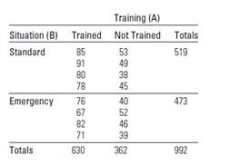
To calculate: ANOVA table

Answer to Problem 11.55E

Source	dF	SS	MS	F
Training	1	4489.00	4489.00	117.49
Situation	1	132.25	132.25	3.46
Interaction	1	56.25	56.25	1.47
Error	12	458.50	38.21
Total	15	5136.00

Explanation of Solution

Given:

Calculation:

  $\begin{array}{l}{\left(AB\right)}_{11}=\text{sum of values in trained column for standard situation =334}\\ {\left(AB\right)}_{12}\text{=sum of values in not trained column for standard situation=185}\\ {\left(AB\right)}_{21}\text{=sum of values in trained column for emergency situation=296 }\\ {\left(AB\right)}_{22}\text{=sum of values in not trained column for emergency situation=177}\end{array}$

Therefore,

  $\begin{array}{l}{A}_1={\left(AB\right)}_{11}+{\left(AB\right)}_{12}=519\\ A_2={\left(AB\right)}_{21}+{\left(AB\right)}_{22}=473\\ B_1={\left(AB\right)}_{11}+{\left(AB\right)}_{21}=630\\ B_2={\left(AB\right)}_{12}+{\left(AB\right)}_{22}=362\end{array}$

  $\begin{array}{l}{\displaystyle \sum x=}{A}_1+A_2=992\\ {\displaystyle \sum x^2=\text{ sum of squares all the data=66640}}\end{array}$

Value of total SS is,

Total $SS={\displaystyle \sum x^2-\frac{{\left({\displaystyle \sum x}\right)}^2}{abr}}=66640-\frac{{\left(999\right)}^2}{2\cdot 2\cdot 4}\approx 5136$

Value of the sum of the squares of factor A is,

  $\begin{array}{c}SSA=\frac{{\left({\displaystyle \sum A_i}\right)}^2}{br}-\frac{{\left({\displaystyle \sum x}\right)}^2}{nbr}\\ =\frac{{\left(519\right)}^2}{2\cdot 4}+\frac{{\left(573\right)}^2}{2\cdot 4}-\frac{{\left(999\right)}^2}{2\cdot 2\cdot 4}\\ \approx 132.25\end{array}$

Value of the sum of the squares of factor B is,

  $\begin{array}{c}SSB=\frac{{\left({\displaystyle \sum B_i}\right)}^2}{br}-\frac{{\left({\displaystyle \sum x}\right)}^2}{nbr}\\ =\frac{{\left(630\right)}^2}{2\cdot 4}+\frac{{\left(360\right)}^2}{2\cdot 4}-\frac{{\left(999\right)}^2}{2\cdot 2\cdot 4}\\ \approx 4489\end{array}$

Value of the sum of the squares of factor A and B is,

  $\begin{array}{c}SS(AB)=\frac{{\left({\displaystyle \sum A{B}_i}\right)}^2}{br}-\frac{{\left({\displaystyle \sum x}\right)}^2}{nbr}\\ =\frac{{\left(334\right)}^2}{4}+\frac{{\left(185\right)}^2}{4}\frac{{\left(296\right)}^2}{4}+\frac{{\left(177\right)}^2}{4}-\frac{{\left(999\right)}^2}{2\cdot 2\cdot 4}-132.25-4489\\ \approx 56.25\end{array}$

Hence,

  $\begin{array}{l}SSE=\text{total SS-}SSA-SSB-SS(AB)\\ =5136-132.25-4489-56.25=458.5\end{array}$

  $d{f}_A$ is the number of levels of factor A decreases by 1

  $\begin{array}{c}d{f}_A=a-1\\ =2-1\\ =1\end{array}$

  $d{f}_B$ is the number of levels of factor B decreased by 1

  $\begin{array}{c}d{f}_B=b-1\\ =2-1\\ =1\end{array}$

  $d{f}_{AB}$ is the product of $d_A$ and $d_B$

  $\begin{array}{c}d{f}_{AB}=d_A{d}_B\\ =\left(1\right)\left(1\right)\\ =1\end{array}$

  $d{f}_E$ is the product of the number of levels of each factor and the number of replications per treatment decrease by 1

  $\begin{array}{c}d{f}_E=ab(r-1)\\ =\left(2\right)\left(2\right)\left(4-1\right)\\ =12\end{array}$

  $\text{total }df$ is the sum of the separate degrees of freedom $d{f}_A$ , $d{f}_B$ , $d{f}_{AB}$ and $d{f}_E$

  $\begin{array}{l}\text{total }df=d{f}_A+d{f}_B+d{f}_{AB}+d{f}_E\\ =1+1+1+12=15\end{array}$

MSA is SSA divided by $d{f}_A$ :

  $\begin{array}{c}MSA=\frac{SSA}{d{f}_A}\\ =\frac{132.25}{1}\\ =132.25\end{array}$

MSB is SSB divided by $d{f}_B$ :

  $\begin{array}{c}MSB=\frac{SSB}{d{f}_B}\\ =\frac{4489}{1}\\ =4489\end{array}$

MS(AB) is SS(AB) divided by $d{f}_{AB}$ :

  $\begin{array}{c}MS(AB)=\frac{SS\left(AB\right)}{d{f}_{AB}}\\ =\frac{56.25}{1}\\ =56.25\end{array}$

MSE is SSE divided by $d{f}_E$ :

  $\begin{array}{c}MSE=\frac{SSE}{d{f}_E}\\ =\frac{458.5}{12}\\ =38.21\end{array}$

The value of the test statistic F is then MST divided by MSE:

  $\begin{array}{c}{F}_A=\frac{MSA}{MSE}\\ =\frac{132.25}{38.21}\\ \approx 3.46\\ F_B=\frac{MSB}{MSE}\\ =\frac{4489}{38.21}\\ \approx 117.49\\ F_{AB}=\frac{MS\left(AB\right)}{MSE}\\ =\frac{56.25}{38.21}\\ \approx 1.47\end{array}$

Source	dF	SS	MS	F
Training	1	4489.00	4489.00	117.49
Situation	1	132.25	132.25	3.46
Interaction	1	56.25	56.25	1.47
Error	12	458.50	38.21
Total	15	5136.00

(b)

To determine

To calculate: is there a significant interaction between the presence or absence of training and the type of decision making situation.

Answer to Problem 11.55E

  $S=6.181R-sq=91.07\%R-sq(adj)=88.84\%$

Explanation of Solution

Given:

Data observations given in exercise 11.54

Calculation:

Now, we want to test the data provide sufficient interaction between the presence of absence of training and the type of decision-making situation using $\alpha =0.05$

Now, test the hypotheses.

The null hypothesis:

  $H_0:$ Factors $A$ and $B$ do not interact.

Versus the alternative hypothesis:

  $H_{\alpha }:$ Factors $\text{A}$ and $\text{B}$ interact.

The test statistic is given by,

  $F=\frac{MS(AB)}{MSE}$

Where $F$ is based on,

  $d{f}_1=(a-1)(b-1)=1(1)=1$

  $d{f}_2=ab(r-1)=2(2)(3)=12$

  $F=\frac{MS(AB)}{MSE}$

  $=\frac{56.25}{38.21}$

  $=1.472$

Rejection region:

Using the critical value approach with $\alpha =0.05,$ we can reject $H_0$ if $F<F_{0.05}=4.75,$ by using $\text{F}$ tabulated values.

since the observed value, $F=1.472,$ do not exceed the critical value. We do not reject $H_0$

No, there is no sufficient evidence to indicate that the two factors $A$ and $B$ interact. So, we need to test the significance for each of the factors independently.

Conclusion:

Therefore, $S=6.181R-sq=91.07\%R-sq(adj)=88.84\%$ .

(c)

To determine

To calculate: whether there is a difference in behaviour ratings for two types of situation at 5% level of significance.

Answer to Problem 11.55E

There is no sufficient evidence to indicate that at least two of the factor a means differ.

Explanation of Solution

Given:

Data observations given in exercise 11.54

Calculation:

Now, we want to test the data provide sufficient evidence to indicate a significance difference in

behavior ratings for the two types of situations at the $5\%$ level of significance or not

Now, test the hypotheses,

  $H_0:$ There are no differences among the factor a means.

Versus the alternative hypothesis

  $H_a:$ At least two of the factor a means differ.

The test statistic is given by,

  $F=\frac{MSA}{MSE}$

Where $F$ is based on

  $d{f}_1=(a-1)=(2-1)=1$

  $d{f}_2=ab(r-1)=2(2)(3)=12$

We have given,

  $\text{MSA}=132.25$

  $\text{MSE}=38.21$

The test statistic is given by,

  $F=\frac{132.25}{38.21}$

  $=3.461135828$

  $\approx 3.46$

Rejection region:

Using the critical value approach with $\alpha =0.05,$ we can reject $H_0,$ if $F>F_{0.05}=161.5,$ by using F tabulated values.

since the observed value, $\text{F}=3.46,$ do not exceed the critical value. We do not reject $H_0.$

Conclusion:

Therefore, there is no sufficient evidence to indicate that at least two of the factor a means differ.

(c)

To determine

To calculate: Whether there is a difference in behavior ratings for two types of the situation at 5% level of significance.

Answer to Problem 11.55E

There is no sufficient evidence to indicate that at least two of the factor a means differ.

Explanation of Solution

Given:

Data observations given in exercise 11.54

Calculation:

Now, we want to test the data provide sufficient evidence to indicate a significant difference in

behavior ratings for the two types of situations at the $5\%$ level of significance or not

Now, test the hypotheses,

  $H_0:$ There are no differences between the factor a means.

Versus the alternative hypothesis

  $H_a:$ At least two of the factor a means differ.

The test statistic is given by,

  $F=\frac{MSA}{MSE}$

Where $F$ is based on

  $d{f}_1=(a-1)=(2-1)=1$

  $d{f}_2=ab(r-1)=2(2)(3)=12$

We have given,

  $\text{MSA}=132.25$

  $\text{MSE}=38.21$

The test statistic is given by,

  $F=\frac{132.25}{38.21}$

  $=3.461135828$

  $\approx 3.46$

Rejection region:

Using the critical value approach with $\alpha =0.05,$ we can reject $H_0,$ if $F>F_{0.05}=161.5,$ by using F tabulated values.

since the observed value, $\text{F}=3.46,$ do not exceed the critical value. We do not reject $H_0.$

Conclusion:

Therefore, there is no sufficient evidence to indicate that at least two of the factor a means differ.

(d)

To determine

To calculate: whether there is a difference in behaviour ratings for two types of situation at 5% level of significance.

Answer to Problem 11.55E

There is sufficient evidence to indicate that at least two of the factor b means differ.

Explanation of Solution

Given:

Data observations are given in exercise 11.54

Calculation:

Now, we want to test the data provide sufficient evidence to indicate a significant for the two types of training categories at the $5\%$ level of significance or not.

Now, test the hypotheses,

  $H_0:$ There are no differences among the factor b means.

Versus the alternative hypothesis

  $H_a:$ At least two of the factor b means differ.

The test statistic is given by,

  $F=\frac{MSB}{MSE}$

Where $F$ is based on

  $d{f}_1=(a-1)=(2-1)=1$

  $d{f}_2=ab(r-1)=2(2)(3)=12$

We have given,

  $\text{MST}=4489$

  $\text{MSE}=38.21$

The test statistic is given by,

  $F=\frac{4489}{38.21}$

  $=117.4823345$

  $\approx 117.48$

Rejection region:

Using the critical value approach with $\alpha =0.05,$ we can reject $H_0$ if $F>F_{0.05}=4.75,$ by using

F tabulated values.

since the observed value, $\text{F}=117.48,$ exceeds the critical value. We reject $H_{\text{o}-}$

Conclusion:

Therefore, there is sufficient evidence to indicate that at least two of the factor b means differ.

(e)

To determine

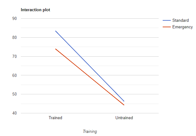
To plot: the average scores using an interaction plot

Answer to Problem 11.55E

Average score plot is drawn

The mean response is higher for the trained supervisors compared to the untrained supervisors, while the mean response appears to be slightly higher overall for the standard situation.

Explanation of Solution

Given:

Data observations are given in exercise 11.54

Calculation:

Therefore, there is no relationship between the two factors $A$ and $B$ . And the main effect $A$ is not significant but the factor $\text{B}$ is significant. since there is no interaction exists between the factors A and $\text{B}$ . We may not produce the average effect of training and the emergency situation on the decision-making abilities of the supervisors.

Conclusion:

Therefore, Average score plot is drawn

The mean response is higher for the trained supervisors compared to the untrained supervisors, while the mean response appears to be slightly higher overall for the standard situation.