
a.
Find the value of b1.
a.
Answer to Problem 16E
The slope b1 is –0.154.
Explanation of Solution
Calculation:
The given information is that the sample data consists of 8 values for x and y.
Slope or b1:
b1=rsysx
where,
r represents the
sy represents the standard deviation of y.
sx represents the standard deviation of x.
Software procedure:
Step-by-step procedure to find the mean, standard deviation for x and y values using MINITAB is given below:
- • Choose Stat > Basic Statistics > Display
Descriptive Statistics . - • In Variables enter the columns of x and y.
- • Choose Options Statistics, and select Mean and Standard deviation.
- • Click OK.
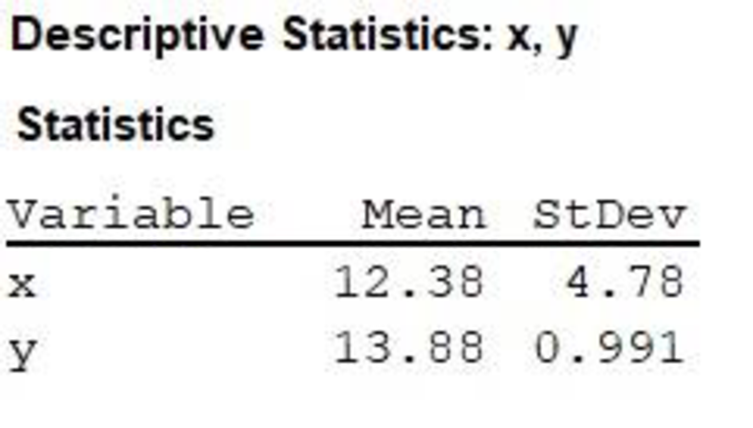
Output obtained from MINITAB is given below:
Correlation:
r=1n−1∑(x−ˉxsx)(y−ˉysy)
The table shows the calculation of correlation:
| x | y | x−ˉx | y−ˉy | x−ˉxsx | y−ˉysy | (x−ˉxsx)(y−ˉysy) |
| 12 | 13 | –0.38 | –0.88 | –0.0795 | –0.888 | 0.0706 |
| 17 | 14 | 4.62 | 0.12 | 0.96653 | 0.12109 | 0.117 |
| 3 | 16 | –9.38 | 2.12 | –1.9623 | 2.13925 | –4.1979 |
| 17 | 13 | 4.62 | –0.88 | 0.96653 | –0.888 | –0.8583 |
| 16 | 14 | 3.62 | 0.12 | 0.75732 | 0.12109 | 0.0917 |
| 11 | 14 | –1.38 | 0.12 | –0.2887 | 0.12109 | –0.035 |
| 14 | 13 | 1.62 | –0.88 | 0.33891 | –0.888 | –0.301 |
| 9 | 14 | –3.38 | 0.12 | –0.7071 | 0.12109 | –0.0856 |
| Total | –5.1985 |
Thus, the correlation is
r=−5.19858−1=−5.19857=−0.743
b1=rsysx
Substitute r as –0.743, sy as 0.991 and sx as 4.78.
b1=−0.743(0.9914.78)=−0.743(0.207)=−0.154
Thus, the slope b1 is –0.154.
b.
Find the residual standard deviation se.
b.
Answer to Problem 16E
The residual standard deviation se is 0.717.
Explanation of Solution
Calculation:
Finding the value of the intercept term before find the residual standard deviation:
Intercept or b0:
b0=ˉy−b1ˉx
ˉy represents the mean of y values.
ˉx represents the mean of x values.
b1 represents the slope coefficient.
Substitute ˉy as 13.88, ˉx as 12.38 and b1 as –0.154.
b0=13.88−(−0.154)(12.38)=13.88+(0.154)(12.38)=13.88+1.91=15.79
Thus, the intercept b0 is 15.79.
The residual standard deviation se is calculated using the formula,
se=√∑(y−ˆy)2n−2
Where,
∑(y−ˆy)2 represents the sum of squares due to error
n represents the sample size.
Thus, the estimated regression equation is ˆy=15.79−0.154x
Use the estimated regression equation to find the predicted value of y for each value of x.
| x | y | ˆy | y−ˆy | (y−ˆy)2 |
| 12 | 13 | 13.942 | –0.942 | 0.88736 |
| 17 | 14 | 13.172 | 0.828 | 0.68558 |
| 3 | 16 | 15.328 | 0.672 | 0.45158 |
| 17 | 13 | 13.172 | –0.172 | 0.02958 |
| 16 | 14 | 13.326 | 0.674 | 0.45428 |
| 11 | 14 | 14.096 | –0.096 | 0.00922 |
| 14 | 13 | 13.634 | –0.634 | 0.40196 |
| 9 | 14 | 14.404 | –0.404 | 0.16322 |
| Total | 3.083 |
Substitute ∑(y−ˆy)2 as 3.083 and n as 8.
se=√3.0838−2=√3.0836=√0.514=0.717
Thus, the residual standard deviation se is 0.717.
c.
Find the sum of squares for x.
c.
Answer to Problem 16E
The sum of squares for x is 159.88.
Explanation of Solution
Calculation:
The table shows the calculation of sum of squares for x
| x | x−ˉx | (x−ˉx)2 |
| 12 | –0.38 | 0.1444 |
| 17 | 4.62 | 21.3444 |
| 3 | –9.38 | 87.9844 |
| 17 | 4.62 | 21.3444 |
| 16 | 3.62 | 13.1044 |
| 11 | –1.38 | 1.9044 |
| 14 | 1.62 | 2.6244 |
| 9 | –3.38 | 11.4244 |
| Total | 159.88 |
Thus, the sum of squares for x is 159.88.
d.
Find the standard error of b1,sb.
d.
Answer to Problem 16E
The standard error of b1, sb is 0.057.
Explanation of Solution
Calculation:
The standard error of b1 is calculated by using the formula:
sb=se√∑(x−ˉx)2
Where,
se represents the residual standard deviation.
∑(x−ˉx)2 represents the sum of squares due to x.
Substitute ∑(x−ˉx)2 as 159.88 and se as 0.717.
sb=0.717√159.88=0.71712.64=0.057
Thus, the standard error of b1, sb is 0.057.
e.
Find the critical value for a 95% confidence interval of β1.
e.
Answer to Problem 16E
The critical value for a 95% confidence interval of β1 is 2.447.
Explanation of Solution
Calculation:
Critical value:
Software procedure:
Step-by-step procedure to find the critical value using MINITAB is given below:
- • Choose Graph > Probability Distribution Plot choose View Probability > OK.
- • From Distribution, choose ‘t’ distribution.
- • In Degrees of freedom, enter 6.
- • Click the Shaded Area tab.
- • Choose Probability and Two tail for the region of the curve to shade.
- • Enter the Probability value as 0.05.
- • Click OK.
Output obtained from MINITAB is given below:
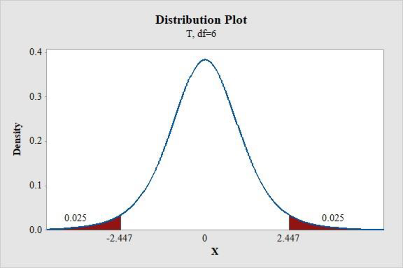
Thus, the critical value for a 95% confidence interval of β1 is 2.447.
f.
Find the margin of error for a 95% confidence interval of β1.
f.
Answer to Problem 16E
The margin of error of b1 is 0.139.
Explanation of Solution
Calculation:
The margin of error for a 95% confidence interval of β1 is calculated using the formula:
Margin of error=tα2⋅sb1
Where,
tα2 represents the two tailed critical value for a given level of significance.
sb1 represents the standard error of b1.
Substitute tα2 as 2.447 and sb1 as 0.057.
Margin of error=(2.447)(0.057)=0.139
Thus, the margin of error of b1 is 0.139.
g.
Construct the 95% confidence interval for β1.
g.
Answer to Problem 16E
The 95% confidence interval for β1 is (−0.293,−0.015)
Explanation of Solution
Calculation:
The confidence interval for β1 is calculated by using the formula:
Confidence interval=b1±tα2⋅sb1
Where,
b1 represents the estimated slope coefficient.
tα2⋅sb1 represents the margin of error.
Confidence interval=−0.154±(2.447)⋅(0.057)=−0.154±0.139=−0.293,−0.015
Thus, the 95% confidence interval for β1 is (−0.293,−0.015)
h.
Test the significance of β1 using 5% level of significance.
h.
Answer to Problem 16E
There is a support of evidence to conclude that there is a linear relationship between x and y at 5% level of significance.
Explanation of Solution
Calculation:
The hypotheses used for testing the significance is given below:
Null hypothesis:
H0:β1=0
That is, there is no linear relationship between x and y.
Alternate hypothesis:
H1:β1≠0
That is, there is a linear relationship between x and y.
Test statistic:
t=ˆβ1−β1sb1
Where,
ˆβ1 represents the estimated slope coefficient.
β1 represents the hypothesized value of slope coefficient.
sb1 represents the standard error of slope coefficient.
Substitute ˆβ1 as –0.154, β1 as 0 and sb1 as 0.057.
t=−0.154−00.057=−0.1540.057=−2.70
From part e, the critical value is identified as –2.447.
Decision Rule:
If the positive test statistic value is greater than or equal to the positive critical value or less than the negative critical value, then reject the null hypothesis. Otherwise do not reject the null hypothesis.
Conclusion:
The test statistic value is –2.70 and the critical value is –2.447.
The test statistic value is lesser than the critical value.
That is, −2.70(=test statistic)<−2.447(=critical value)
Thus, the null hypothesis is rejected.
Hence, there is a support of evidence to conclude that there is a linear relationship between x and y.
Want to see more full solutions like this?
Chapter 11 Solutions
ALEKS 360 ESSENT. STAT ACCESS CARD

- For a binary asymmetric channel with Py|X(0|1) = 0.1 and Py|X(1|0) = 0.2; PX(0) = 0.4 isthe probability of a bit of “0” being transmitted. X is the transmitted digit, and Y is the received digit.a. Find the values of Py(0) and Py(1).b. What is the probability that only 0s will be received for a sequence of 10 digits transmitted?c. What is the probability that 8 1s and 2 0s will be received for the same sequence of 10 digits?d. What is the probability that at least 5 0s will be received for the same sequence of 10 digits?arrow_forwardV2 360 Step down + I₁ = I2 10KVA 120V 10KVA 1₂ = 360-120 or 2nd Ratio's V₂ m 120 Ratio= 360 √2 H I2 I, + I2 120arrow_forwardQ2. [20 points] An amplitude X of a Gaussian signal x(t) has a mean value of 2 and an RMS value of √(10), i.e. square root of 10. Determine the PDF of x(t).arrow_forward
- In a network with 12 links, one of the links has failed. The failed link is randomlylocated. An electrical engineer tests the links one by one until the failed link is found.a. What is the probability that the engineer will find the failed link in the first test?b. What is the probability that the engineer will find the failed link in five tests?Note: You should assume that for Part b, the five tests are done consecutively.arrow_forwardProblem 3. Pricing a multi-stock option the Margrabe formula The purpose of this problem is to price a swap option in a 2-stock model, similarly as what we did in the example in the lectures. We consider a two-dimensional Brownian motion given by W₁ = (W(¹), W(2)) on a probability space (Q, F,P). Two stock prices are modeled by the following equations: dX = dY₁ = X₁ (rdt+ rdt+0₁dW!) (²)), Y₁ (rdt+dW+0zdW!"), with Xo xo and Yo =yo. This corresponds to the multi-stock model studied in class, but with notation (X+, Y₁) instead of (S(1), S(2)). Given the model above, the measure P is already the risk-neutral measure (Both stocks have rate of return r). We write σ = 0₁+0%. We consider a swap option, which gives you the right, at time T, to exchange one share of X for one share of Y. That is, the option has payoff F=(Yr-XT). (a) We first assume that r = 0 (for questions (a)-(f)). Write an explicit expression for the process Xt. Reminder before proceeding to question (b): Girsanov's theorem…arrow_forwardProblem 1. Multi-stock model We consider a 2-stock model similar to the one studied in class. Namely, we consider = S(1) S(2) = S(¹) exp (σ1B(1) + (M1 - 0/1 ) S(²) exp (02B(2) + (H₂- M2 where (B(¹) ) +20 and (B(2) ) +≥o are two Brownian motions, with t≥0 Cov (B(¹), B(2)) = p min{t, s}. " The purpose of this problem is to prove that there indeed exists a 2-dimensional Brownian motion (W+)+20 (W(1), W(2))+20 such that = S(1) S(2) = = S(¹) exp (011W(¹) + (μ₁ - 01/1) t) 롱) S(²) exp (021W (1) + 022W(2) + (112 - 03/01/12) t). where σ11, 21, 22 are constants to be determined (as functions of σ1, σ2, p). Hint: The constants will follow the formulas developed in the lectures. (a) To show existence of (Ŵ+), first write the expression for both W. (¹) and W (2) functions of (B(1), B(²)). as (b) Using the formulas obtained in (a), show that the process (WA) is actually a 2- dimensional standard Brownian motion (i.e. show that each component is normal, with mean 0, variance t, and that their…arrow_forward
- The scores of 8 students on the midterm exam and final exam were as follows. Student Midterm Final Anderson 98 89 Bailey 88 74 Cruz 87 97 DeSana 85 79 Erickson 85 94 Francis 83 71 Gray 74 98 Harris 70 91 Find the value of the (Spearman's) rank correlation coefficient test statistic that would be used to test the claim of no correlation between midterm score and final exam score. Round your answer to 3 places after the decimal point, if necessary. Test statistic: rs =arrow_forwardBusiness discussarrow_forwardBusiness discussarrow_forward
 MATLAB: An Introduction with ApplicationsStatisticsISBN:9781119256830Author:Amos GilatPublisher:John Wiley & Sons Inc
 Probability and Statistics for Engineering and th...StatisticsISBN:9781305251809Author:Jay L. DevorePublisher:Cengage Learning
 Statistics for The Behavioral Sciences (MindTap C...StatisticsISBN:9781305504912Author:Frederick J Gravetter, Larry B. WallnauPublisher:Cengage Learning
 Elementary Statistics: Picturing the World (7th E...StatisticsISBN:9780134683416Author:Ron Larson, Betsy FarberPublisher:PEARSON
 The Basic Practice of StatisticsStatisticsISBN:9781319042578Author:David S. Moore, William I. Notz, Michael A. FlignerPublisher:W. H. Freeman
 Introduction to the Practice of StatisticsStatisticsISBN:9781319013387Author:David S. Moore, George P. McCabe, Bruce A. CraigPublisher:W. H. Freeman