
a.
Find the point estimates
a.
Answer to Problem 15CQ
The intercept
The slope
Explanation of Solution
Calculation:
The given information is that the sample data consists of 8 values for x and y.
Slope or
where,
r represents the
Software procedure:
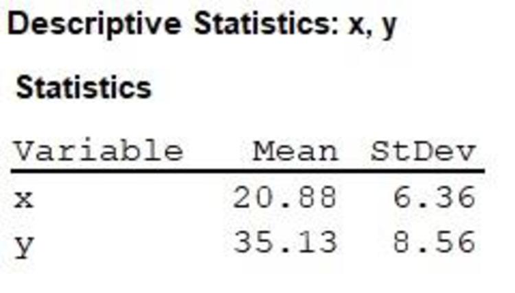
Step-by-step procedure to find the mean, standard deviation for x and y values using MINITAB is given below:
- • Choose Stat > Basic Statistics > Display
Descriptive Statistics . - • In Variables enter the columns of y and x.
- • Choose Options Statistics, select Mean and Standard deviation.
- • Click OK.
Output obtained from MINITAB is given below:
Correlation:
Where,
n represents the sample size.
The table shows the calculation of correlation:
| x | y | | ||||
| 25 | 40 | 4.12 | 4.87 | 0.6478 | 0.56893 | 0.36855 |
| 13 | 20 | –7.88 | –15.13 | –1.239 | –1.7675 | 2.18995 |
| 16 | 33 | –4.88 | –2.13 | –0.7673 | –0.2488 | 0.19093 |
| 19 | 30 | –1.88 | –5.13 | –0.2956 | –0.5993 | 0.17715 |
| 29 | 50 | 8.12 | 14.87 | 1.27673 | 1.73715 | 2.21787 |
| 19 | 37 | –1.88 | 1.87 | –0.2956 | 0.21846 | –0.0646 |
| 16 | 34 | –4.88 | –1.13 | –0.7673 | –0.132 | 0.10129 |
| 30 | 37 | 9.12 | 1.87 | 1.43396 | 0.21846 | 0.31326 |
| Total | 5.4944 |
Thus, the correlation is
Substitute r as 0.7850,
Thus, the slope
Intercept of
Substitute
Thus, the intercept
b.
Construct the 95% confidence interval for
b.
Answer to Problem 15CQ
The 95% confidence interval for
Explanation of Solution
Calculation:
The confidence interval for
Where,
Critical value:
Software procedure:
Step-by-step procedure to find the critical value using MINITAB is given below:
- • Choose Graph > Probability Distribution Plot choose View Probability > OK.
- • From Distribution, choose ‘t’ distribution.
- • In Degrees of freedom, enter 6.
- • Click the Shaded Area tab.
- • Choose Probability and Two tail for the region of the curve to shade.
- • Enter the Probability value as 0.05.
- • Click OK.
Output obtained from MINITAB is given below:
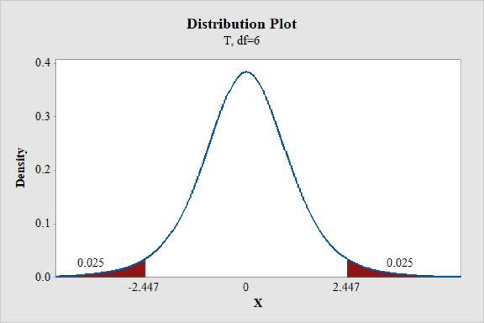
Thus, the critical value for a 95% confidence interval of
The standard error of
Where,
Calculation of residual standard deviation:
Use the estimated regression equation to find the predicted value of y for each value of x and the estimated regression equation is
The table below shows the calculation of residual standard deviation:
| x | y | |||
| 25 | 40 | 39.5 | 0.5 | 0.25 |
| 13 | 20 | 26.78 | –6.78 | 45.9684 |
| 16 | 33 | 29.96 | 3.04 | 9.2416 |
| 19 | 30 | 33.14 | -3.14 | 9.8596 |
| 29 | 50 | 43.74 | 6.26 | 39.1876 |
| 19 | 37 | 33.14 | 3.86 | 14.8996 |
| 16 | 34 | 29.96 | 4.04 | 16.3216 |
| 30 | 37 | 44.8 | –7.8 | 60.84 |
| Total | 196.57 |
Substitute
Thus, the residual standard deviation
The table shows the calculation of sum of squares for x.
| x | ||
| 25 | 4.12 | 16.9744 |
| 13 | –7.88 | 62.0944 |
| 16 | –4.88 | 23.8144 |
| 19 | –1.88 | 3.5344 |
| 29 | 8.12 | 65.9344 |
| 19 | –1.88 | 3.5344 |
| 16 | –4.88 | 23.8144 |
| 30 | 9.12 | 83.1744 |
| Total | 282.88 |
Substitute
Thus, the standard error of
95% confidence interval for
Thus, the 95% confidence interval for
c.
Test the significance of
c.
Answer to Problem 15CQ
There is no support of evidence to conclude that there is a linear relationship between x and y at 1% level of significance.
Explanation of Solution
Calculation:
The hypotheses used for testing the significance is given below:
Null hypothesis:
That is, there is no linear relationship between x and y.
Alternate hypothesis:
That is, there is a linear relationship between x and y.
Test statistic:
Where,
Substitute
Critical value:
Software procedure:
Step-by-step procedure to find the critical value using MINITAB is given below:
- • Choose Graph > Probability Distribution Plot choose View Probability > OK.
- • From Distribution, choose ‘t’ distribution.
- • In Degrees of freedom, enter 6.
- • Click the Shaded Area tab.
- • Choose Probability and Two tail for the region of the curve to shade.
- • Enter the Probability value as 0.01.
- • Click OK.
Output obtained from MINITAB is given below:
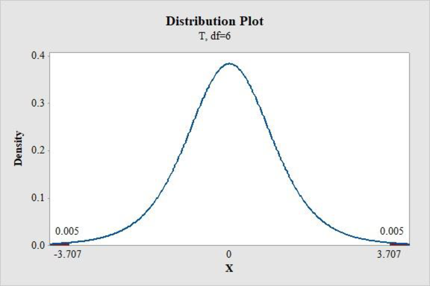
Thus, the critical value for a 99% confidence interval of
Decision Rule:
Reject the null hypothesis when the test statistic value is greater than the critical value for a given level of significance. Otherwise, do not reject the null hypothesis.
Conclusion:
The test statistic value is 3.12 and the critical value is 3.707.
The test statistic value is lesser than the critical value.
That is,
Thus, the null hypothesis is not rejected.
Hence, there is no support of evidence to conclude that there is a linear relationship between x and y at 1% level of significance.
d.
Construct the 95% confidence interval for the mean response for the given value of x.
d.
Answer to Problem 15CQ
The 95% confidence interval for the mean response for the given value of x is
Explanation of Solution
Calculation:
The given value of x is 20.
Software procedure:
Step-by-step procedure to construct the 95% confidence interval for the mean response for the given value of x is given below:
- • Choose Stat > Regression > Regression.
- • In Response, enter the column containing the y.
- • In Predictors, enter the columns containing the x.
- • Click OK.
- • Choose Stat > Regression > Regression>Predict.
- • Choose Enter the individual values.
- • Enter the x as 20.
- • Click OK.
Output obtained from MINITAB is given below:
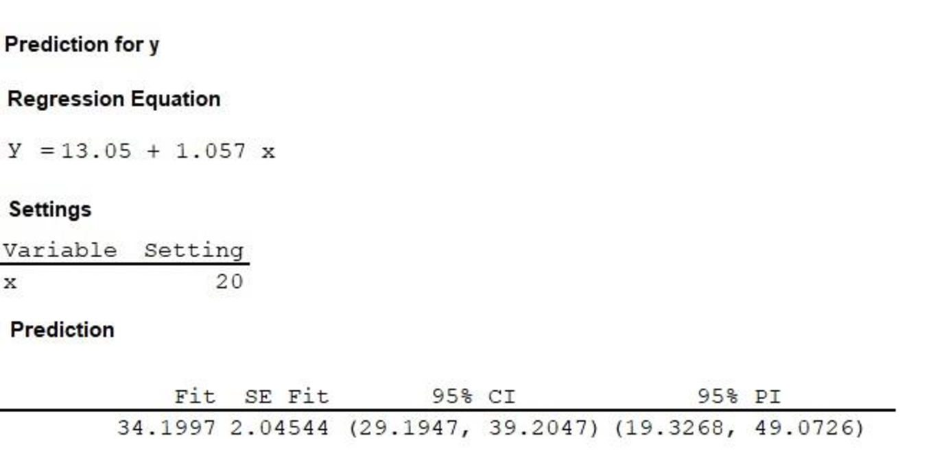
Interpretation:
Thus, the 95% confidence interval for the mean response for the given value of x is
e.
Construct the 95% prediction interval for the individual response for the given value of x.
e.
Answer to Problem 15CQ
The 95% prediction interval for the individual response for the given value of x is
Explanation of Solution
The given value of x is 20.
From the MINITAB output obtained in the previous part (d) it can be observed that the 95% prediction interval for the individual response for the given value of x is
Want to see more full solutions like this?
Chapter 11 Solutions
ALEKS 360 ESSENT. STAT ACCESS CARD

- Questions An insurance company's cumulative incurred claims for the last 5 accident years are given in the following table: Development Year Accident Year 0 2018 1 2 3 4 245 267 274 289 292 2019 255 276 288 294 2020 265 283 292 2021 263 278 2022 271 It can be assumed that claims are fully run off after 4 years. The premiums received for each year are: Accident Year Premium 2018 306 2019 312 2020 318 2021 326 2022 330 You do not need to make any allowance for inflation. 1. (a) Calculate the reserve at the end of 2022 using the basic chain ladder method. (b) Calculate the reserve at the end of 2022 using the Bornhuetter-Ferguson method. 2. Comment on the differences in the reserves produced by the methods in Part 1.arrow_forwardA population that is uniformly distributed between a=0and b=10 is given in sample sizes 50( ), 100( ), 250( ), and 500( ). Find the sample mean and the sample standard deviations for the given data. Compare your results to the average of means for a sample of size 10, and use the empirical rules to analyze the sampling error. For each sample, also find the standard error of the mean using formula given below. Standard Error of the Mean =sigma/Root Complete the following table with the results from the sampling experiment. (Round to four decimal places as needed.) Sample Size Average of 8 Sample Means Standard Deviation of 8 Sample Means Standard Error 50 100 250 500arrow_forwardA survey of 250250 young professionals found that two dash thirdstwo-thirds of them use their cell phones primarily for e-mail. Can you conclude statistically that the population proportion who use cell phones primarily for e-mail is less than 0.720.72? Use a 95% confidence interval. Question content area bottom Part 1 The 95% confidence interval is left bracket nothing comma nothing right bracket0.60820.6082, 0.72510.7251. As 0.720.72 is within the limits of the confidence interval, we cannot conclude that the population proportion is less than 0.720.72. (Use ascending order. Round to four decimal places as needed.)arrow_forward
- I need help with this problem and an explanation of the solution for the image described below. (Statistics: Engineering Probabilities)arrow_forwardA survey of 250 young professionals found that two-thirds of them use their cell phones primarily for e-mail. Can you conclude statistically that the population proportion who use cell phones primarily for e-mail is less than 0.72? Use a 95% confidence interval. Question content area bottom Part 1 The 95% confidence interval is [ ], [ ] As 0.72 is ▼ above the upper limit within the limits below the lower limit of the confidence interval, we ▼ can cannot conclude that the population proportion is less than 0.72. (Use ascending order. Round to four decimal places as needed.)arrow_forwardI need help with this problem and an explanation of the solution for the image described below. (Statistics: Engineering Probabilities)arrow_forward
- I need help with this problem and an explanation of the solution for the image described below. (Statistics: Engineering Probabilities)arrow_forwardI need help with this problem and an explanation of the solution for the image described below. (Statistics: Engineering Probabilities)arrow_forwardQuestions An insurance company's cumulative incurred claims for the last 5 accident years are given in the following table: Development Year Accident Year 0 2018 1 2 3 4 245 267 274 289 292 2019 255 276 288 294 2020 265 283 292 2021 263 278 2022 271 It can be assumed that claims are fully run off after 4 years. The premiums received for each year are: Accident Year Premium 2018 306 2019 312 2020 318 2021 326 2022 330 You do not need to make any allowance for inflation. 1. (a) Calculate the reserve at the end of 2022 using the basic chain ladder method. (b) Calculate the reserve at the end of 2022 using the Bornhuetter-Ferguson method. 2. Comment on the differences in the reserves produced by the methods in Part 1.arrow_forward
- Questions An insurance company's cumulative incurred claims for the last 5 accident years are given in the following table: Development Year Accident Year 0 2018 1 2 3 4 245 267 274 289 292 2019 255 276 288 294 2020 265 283 292 2021 263 278 2022 271 It can be assumed that claims are fully run off after 4 years. The premiums received for each year are: Accident Year Premium 2018 306 2019 312 2020 318 2021 326 2022 330 You do not need to make any allowance for inflation. 1. (a) Calculate the reserve at the end of 2022 using the basic chain ladder method. (b) Calculate the reserve at the end of 2022 using the Bornhuetter-Ferguson method. 2. Comment on the differences in the reserves produced by the methods in Part 1.arrow_forwardFrom a sample of 26 graduate students, the mean number of months of work experience prior to entering an MBA program was 34.67. The national standard deviation is known to be18 months. What is a 90% confidence interval for the population mean? Question content area bottom Part 1 A 9090% confidence interval for the population mean is left bracket nothing comma nothing right bracketenter your response here,enter your response here. (Use ascending order. Round to two decimal places as needed.)arrow_forwardA test consists of 10 questions made of 5 answers with only one correct answer. To pass the test, a student must answer at least 8 questions correctly. (a) If a student guesses on each question, what is the probability that the student passes the test? (b) Find the mean and standard deviation of the number of correct answers. (c) Is it unusual for a student to pass the test by guessing? Explain.arrow_forward
 MATLAB: An Introduction with ApplicationsStatisticsISBN:9781119256830Author:Amos GilatPublisher:John Wiley & Sons Inc
 Probability and Statistics for Engineering and th...StatisticsISBN:9781305251809Author:Jay L. DevorePublisher:Cengage Learning
 Statistics for The Behavioral Sciences (MindTap C...StatisticsISBN:9781305504912Author:Frederick J Gravetter, Larry B. WallnauPublisher:Cengage Learning
 Elementary Statistics: Picturing the World (7th E...StatisticsISBN:9780134683416Author:Ron Larson, Betsy FarberPublisher:PEARSON
 The Basic Practice of StatisticsStatisticsISBN:9781319042578Author:David S. Moore, William I. Notz, Michael A. FlignerPublisher:W. H. Freeman
 Introduction to the Practice of StatisticsStatisticsISBN:9781319013387Author:David S. Moore, George P. McCabe, Bruce A. CraigPublisher:W. H. Freeman