
Videos
The accompanying data resulted from an experiment to investigate whether yield from a certain chemical process depended either on the formulation of a particular input or on mixer speed.
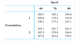
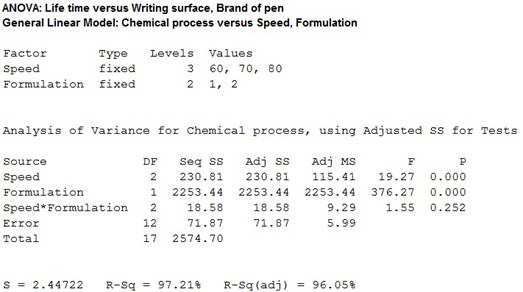
A statistical computer package gave SS(Form) = 2253.44, SS(Speed) = 230.81, SS(Form*Speed) = 18.58, and SSE = 71.87.
a. Does there appear to be interaction between the factors?
b. Does yield appear to depend on either formulation or speed?
c. Calculate estimates of the main effects.
d. The fitted values are
e. Construct a normal
a.
Identify whether there is a significant effect from interaction between speed and formulation.
Answer to Problem 18E
There is no sufficient evidence to conclude that there is an effect of interaction between mix speed and formulation on the chemical process.
Explanation of Solution
Given info:
An experiment was carried out to test the effect of formulation and speed on the chemical press. The formulation has two levels and speed has three levels.
The sum of squares due to formulation is 2,253.44, sum of squares due to speed is 230.81, sum of squares due to error is 71.87, sum of squares due to interaction between formulation and speed is 18.58.
Calculation:
Testing the Hypothesis:
Null hypothesis:
That is, the interaction effect between mix speed and formulation has no significant effect on chemical process.
Alternative hypothesis:
That is, the interaction effect between mix speed and formulation has no significant effect on chemical process.
Test statistic:
Software procedure:
Step by step procedure to find the test statistic using Minitab is given below:
- Choose Stat > ANOVA > General Linear Model.
- In Responses, enter the column of Chemical process.
- In Model, enter the column of Speed, Formulation, Speed*Formulation.
- In Results, choose “Analysis of variance table”.
- Click OK in all dialog boxes.
Output obtained from MINITAB is given below:
Conclusion:
Interaction effect of AB:
The P- value for the interaction effect AB is 0.252 and the level of significance is 0.01.
The P- value is lesser than the level of significance.
That is,
Thus, the null hypothesis is not rejected,
Hence, there is no sufficient evidence to conclude that there is an effect of interaction between mix speed and formulation on the chemical process.
b.
Identify whether the yield of the chemical process depends on speed or formulation.
Answer to Problem 18E
The yield of a chemical process depends on both speed and formulation.
Explanation of Solution
From the MINITAB output obtained in part (a), the following can be observed.
For Main effect of factor A speed:
The P- value for the factor A (speed) is 0.000 and the level of significance is 0.01.
The P- value is lesser than the level of significance.
That is,.
Thus, the null hypothesis is rejected,
Hence, there is sufficient evidence to conclude that there is an effect of speed on the yield of chemical process.
For Main effect of factor B formulation:
The P- value for the factor B (formulation) is 0.000 and the level of significance is 0.01.
The P- value is lesser than the level of significance.
That is,
Thus, the null hypothesis is rejected,
Hence, there is sufficient evidence to conclude that there is an effect of formulation on the yield of chemical process.
c.
Find the estimates for the main effects.
Explanation of Solution
Calculation:
Where,
Overall mean effect:
Mean due to the first level of factor A:
Mean due to the second level of factor A:
Main effect of factor A:
At first level:
At second level:
Mean due to the first level of factor B:
Mean due to the second level of factor B:
Mean due to the third level of factor B
Main effect of factor B:
d.
Verify whether the calculated residuals are equal to the given residual values.
Explanation of Solution
Calculation:
The interaction effect for the first level of factor A and the first level of factor B
The interaction effect for the first level of factor A and the second level of factor B
The interaction effect for the first level of factor A and the third level of factor B
Similarly, the remaining values are given below:
| S. No | Values |
| 1 | |
| 2 | |
| 3 | |
| 4 | |
| 5 | |
| 6 |
The fitted values are calculated by using the formula:
Where,
i represents the levels of factor A.
j represents the levels of factor B.
k represents the observation.
The predicted value when
Similarly, the other fitted values are calculated, the table shows the fitted values:
| S. No | 1 | 2 | 3 | 4 | 5 | 6 | 7 | 8 | 9 |
| Fitted values | 189.47 | 189.47 | 189.47 | 166.20 | 166.20 | 166.20 | 180.60 | 180.60 | 180.60 |
| S. No | 10 | 11 | 12 | 13 | 14 | 15 | 16 | 17 | 18 |
| Fitted values | 161.03 | 161.03 | 161.03 | 191.03 | 191.03 | 191.03 | 166.73 | 166.73 | 166.73 |
The residuals values are calculated by using the formula:
The table shows below gives the residuals for each observation:
| S. No |
Observed |
Fitted values | |
| 1 | 189.7 | 189.47 | 0.23 |
| 2 | 188.6 | 189.47 | –0.87 |
| 3 | 190.1 | 189.47 | 0.63 |
| 4 | 165.1 | 166.20 | –1.1 |
| 5 | 165.9 | 166.20 | –0.3 |
| 6 | 167.6 | 166.20 | 1.4 |
| 7 | 185.1 | 180.60 | 4.5 |
| 8 | 179.4 | 180.60 | –1.2 |
| 9 | 177.3 | 180.60 | –3.3 |
| 10 | 161.7 | 161.03 | 0.67 |
| 11 | 159.8 | 161.03 | –1.23 |
| 12 | 161.6 | 161.03 | 0.57 |
| 13 | 189 | 191.03 | –2.03 |
| 14 | 193 | 191.03 | 1.97 |
| 15 | 191.1 | 191.03 | 0.07 |
| 16 | 163.3 | 166.73 | –3.43 |
| 17 | 166.6 | 166.73 | –0.13 |
| 18 | 170.3 | 166.73 | 3.57 |
Hence, the calculated residuals values are equal to given residual values.
e.
Construct a normal probability plot for the residuals obtained in part (d).
Identify whether the residuals are normally distributed.
Answer to Problem 18E
The normal probability of residuals is given below:
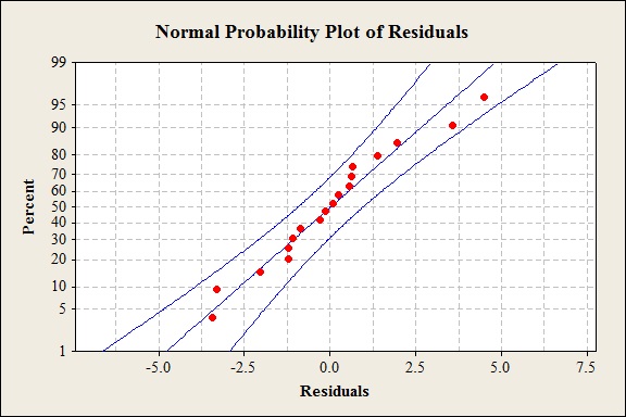
The residuals are normally distributed.
Explanation of Solution
Calculation:
Normal probability plot of residuals:
Software procedure:
Step-by-step procedure to construct a normal probability plot of residuals is given below:
- Click on Graph>Probability plot>Single.
- Click OK.
- Under Graph variables, select the column containing the residual values.
- Click on Distribution and selection Normal.
- Click OK.
Interpretation:
The normal probability plot of residuals suggests that the residuals are normally distributed because the residuals fall approximately on a straight line.
Want to see more full solutions like this?
Chapter 11 Solutions
Student Solutions Manual for Devore's Probability and Statistics for Engineering and the Sciences, 9th


- According to an economist from a financial company, the average expenditures on "furniture and household appliances" have been lower for households in the Montreal area than those in the Quebec region. A random sample of 14 households from the Montreal region and 16 households from the Quebec region was taken, providing the following data regarding expenditures in this economic sector. It is assumed that the data from each population are distributed normally. We are interested in knowing if the variances of the populations are equal. a) Perform the appropriate hypothesis test on two variances at a significance level of 1%. Include the following information: i. Hypothesis / Identification of populations ii. Critical F-value(s) iii. Decision rule iv. F-ratio value v. Decision and conclusion b) Based on the results obtained in a), is the hypothesis of equal variances for this socio-economic characteristic measured in these two populations upheld? c) Based on the results obtained in a),…arrow_forwardA major company in the Montreal area, offering a range of engineering services from project preparation to construction execution, and industrial project management, wants to ensure that the individuals who are responsible for project cost estimation and bid preparation demonstrate a certain uniformity in their estimates. The head of civil engineering and municipal services decided to structure an experimental plan to detect if there could be significant differences in project evaluation. Seven projects were selected, each of which had to be evaluated by each of the two estimators, with the order of the projects submitted being random. The obtained estimates are presented in the table below. a) Complete the table above by calculating: i. The differences (A-B) ii. The sum of the differences iii. The mean of the differences iv. The standard deviation of the differences b) What is the value of the t-statistic? c) What is the critical t-value for this test at a significance level of 1%?…arrow_forwardCompute the relative risk of falling for the two groups (did not stop walking vs. did stop). State/interpret your result verbally.arrow_forward
- Microsoft Excel include formulasarrow_forwardQuestion 1 The data shown in Table 1 are and R values for 24 samples of size n = 5 taken from a process producing bearings. The measurements are made on the inside diameter of the bearing, with only the last three decimals recorded (i.e., 34.5 should be 0.50345). Table 1: Bearing Diameter Data Sample Number I R Sample Number I R 1 34.5 3 13 35.4 8 2 34.2 4 14 34.0 6 3 31.6 4 15 37.1 5 4 31.5 4 16 34.9 7 5 35.0 5 17 33.5 4 6 34.1 6 18 31.7 3 7 32.6 4 19 34.0 8 8 33.8 3 20 35.1 9 34.8 7 21 33.7 2 10 33.6 8 22 32.8 1 11 31.9 3 23 33.5 3 12 38.6 9 24 34.2 2 (a) Set up and R charts on this process. Does the process seem to be in statistical control? If necessary, revise the trial control limits. [15 pts] (b) If specifications on this diameter are 0.5030±0.0010, find the percentage of nonconforming bearings pro- duced by this process. Assume that diameter is normally distributed. [10 pts] 1arrow_forward4. (5 pts) Conduct a chi-square contingency test (test of independence) to assess whether there is an association between the behavior of the elderly person (did not stop to talk, did stop to talk) and their likelihood of falling. Below, please state your null and alternative hypotheses, calculate your expected values and write them in the table, compute the test statistic, test the null by comparing your test statistic to the critical value in Table A (p. 713-714) of your textbook and/or estimating the P-value, and provide your conclusions in written form. Make sure to show your work. Did not stop walking to talk Stopped walking to talk Suffered a fall 12 11 Totals 23 Did not suffer a fall | 2 Totals 35 37 14 46 60 Tarrow_forward
- Question 2 Parts manufactured by an injection molding process are subjected to a compressive strength test. Twenty samples of five parts each are collected, and the compressive strengths (in psi) are shown in Table 2. Table 2: Strength Data for Question 2 Sample Number x1 x2 23 x4 x5 R 1 83.0 2 88.6 78.3 78.8 3 85.7 75.8 84.3 81.2 78.7 75.7 77.0 71.0 84.2 81.0 79.1 7.3 80.2 17.6 75.2 80.4 10.4 4 80.8 74.4 82.5 74.1 75.7 77.5 8.4 5 83.4 78.4 82.6 78.2 78.9 80.3 5.2 File Preview 6 75.3 79.9 87.3 89.7 81.8 82.8 14.5 7 74.5 78.0 80.8 73.4 79.7 77.3 7.4 8 79.2 84.4 81.5 86.0 74.5 81.1 11.4 9 80.5 86.2 76.2 64.1 80.2 81.4 9.9 10 75.7 75.2 71.1 82.1 74.3 75.7 10.9 11 80.0 81.5 78.4 73.8 78.1 78.4 7.7 12 80.6 81.8 79.3 73.8 81.7 79.4 8.0 13 82.7 81.3 79.1 82.0 79.5 80.9 3.6 14 79.2 74.9 78.6 77.7 75.3 77.1 4.3 15 85.5 82.1 82.8 73.4 71.7 79.1 13.8 16 78.8 79.6 80.2 79.1 80.8 79.7 2.0 17 82.1 78.2 18 84.5 76.9 75.5 83.5 81.2 19 79.0 77.8 20 84.5 73.1 78.2 82.1 79.2 81.1 7.6 81.2 84.4 81.6 80.8…arrow_forwardName: Lab Time: Quiz 7 & 8 (Take Home) - due Wednesday, Feb. 26 Contingency Analysis (Ch. 9) In lab 5, part 3, you will create a mosaic plot and conducted a chi-square contingency test to evaluate whether elderly patients who did not stop walking to talk (vs. those who did stop) were more likely to suffer a fall in the next six months. I have tabulated the data below. Answer the questions below. Please show your calculations on this or a separate sheet. Did not stop walking to talk Stopped walking to talk Totals Suffered a fall Did not suffer a fall Totals 12 11 23 2 35 37 14 14 46 60 Quiz 7: 1. (2 pts) Compute the odds of falling for each group. Compute the odds ratio for those who did not stop walking vs. those who did stop walking. Interpret your result verbally.arrow_forwardSolve please and thank you!arrow_forward
- 7. In a 2011 article, M. Radelet and G. Pierce reported a logistic prediction equation for the death penalty verdicts in North Carolina. Let Y denote whether a subject convicted of murder received the death penalty (1=yes), for the defendant's race h (h1, black; h = 2, white), victim's race i (i = 1, black; i = 2, white), and number of additional factors j (j = 0, 1, 2). For the model logit[P(Y = 1)] = a + ß₁₂ + By + B²², they reported = -5.26, D â BD = 0, BD = 0.17, BY = 0, BY = 0.91, B = 0, B = 2.02, B = 3.98. (a) Estimate the probability of receiving the death penalty for the group most likely to receive it. [4 pts] (b) If, instead, parameters used constraints 3D = BY = 35 = 0, report the esti- mates. [3 pts] h (c) If, instead, parameters used constraints Σ₁ = Σ₁ BY = Σ; B = 0, report the estimates. [3 pts] Hint the probabilities, odds and odds ratios do not change with constraints.arrow_forwardSolve please and thank you!arrow_forwardSolve please and thank you!arrow_forward
 Big Ideas Math A Bridge To Success Algebra 1: Stu...AlgebraISBN:9781680331141Author:HOUGHTON MIFFLIN HARCOURTPublisher:Houghton Mifflin Harcourt
 Functions and Change: A Modeling Approach to Coll...AlgebraISBN:9781337111348Author:Bruce Crauder, Benny Evans, Alan NoellPublisher:Cengage Learning
 Glencoe Algebra 1, Student Edition, 9780079039897...AlgebraISBN:9780079039897Author:CarterPublisher:McGraw Hill
 Linear Algebra: A Modern IntroductionAlgebraISBN:9781285463247Author:David PoolePublisher:Cengage Learning
 Holt Mcdougal Larson Pre-algebra: Student Edition...AlgebraISBN:9780547587776Author:HOLT MCDOUGALPublisher:HOLT MCDOUGAL